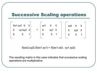
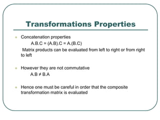
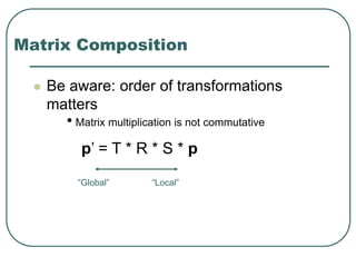
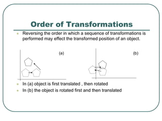
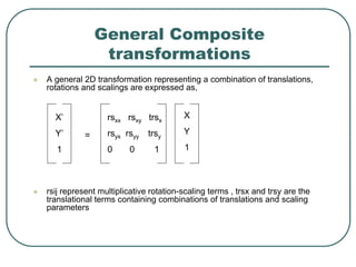
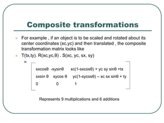
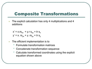
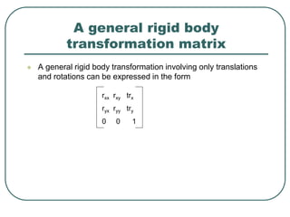
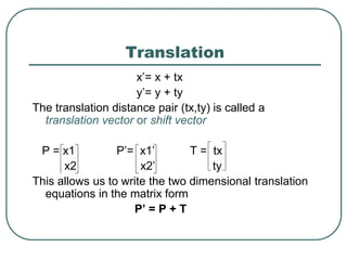
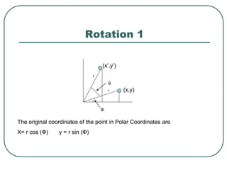
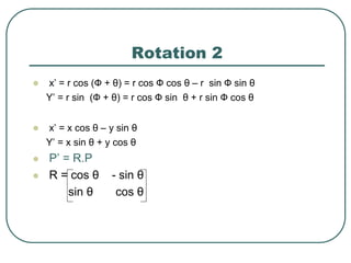
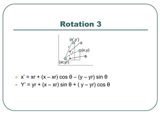
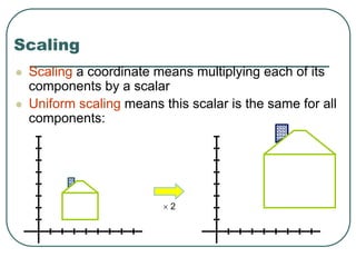
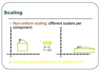
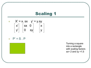
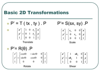
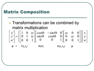
2D transformations can be represented by matrices and include translations, rotations, scalings, and reflections. Translations move objects by adding a translation vector. Rotations rotate objects around the origin by pre-multiplying the point coordinates with a rotation matrix. Scaling enlarges or shrinks objects by multiplying the point coordinates with scaling factors. Composite transformations represent multiple transformations applied in sequence, with the overall transformation represented as the matrix product of the individual transformations. The order of transformations matters as matrix multiplication is not commutative.

1. 2D TRANSFORMATIONS

2. Overview
 2D Transformations
• Basic 2D transformations
• Matrix representation
• Matrix composition

3. Basic 2D transformations
 The basic geometric transformations
are translation, rotation, and scaling.
Other transformations that are often
applied to objects include reflection and
shearing.

4. Translation
x’= x + tx
y’= y + ty
The translation distance pair (tx,ty) is called a
translation vector or shift vector
P = x1 P’= x1’ T = tx
x2 x2’ ty
This allows us to write the two dimensional translation
equations in the matrix form
P’ = P + T

5. Translation Illustration
P’
P

6. Rotation 1
r
r
Ф
(x,y)
(x’,y’)
The original coordinates of the point in Polar Coordinates are
X= r cos (Ф) y = r sin (Ф)
θ

7. Rotation 2
 x’ = r cos (Ф + θ) = r cos Ф cos θ – r sin Ф sin θ
Y’ = r sin (Ф + θ) = r cos Ф sin θ + r sin Ф cos θ
 x’ = x cos θ – y sin θ
Y’ = x sin θ + y cos θ
 P’ = R.P
 R = cos θ - sin θ
sin θ cos θ

8. Rotation 3
 x’ = xr + (x – xr) cos θ – (y – yr) sin θ
 Y’ = yr + (x – xr) sin θ + ( y – yr) cos θ
r
r
Ф
θ
(x,y)
(x’,y’)
(xr,yr)

9. Scaling
 Scaling a coordinate means multiplying each of its
components by a scalar
 Uniform scaling means this scalar is the same for all
components:
 2

10.  Non-uniform scaling: different scalars per
component:
 How can we represent this in matrix form?
Scaling
X  2,
Y  0.5

11. Scaling 1
 X’ = x. sx y’ = y.sy
x’ sx 0 x
y’ 0 sy y
 P’ = S . P
Turning a square
into a rectangle
with scaling factors
sx= 2 and sy =1.5

12. Scaling 2
Using sx= sy = 0.5 the line is
reduced in size and moved
closer to the origin
p1
p2
p3
(xf,yf)
Scaling relative to a chosen fixed point (xf, yf) .
Distances from each polygon vertex to the fixed
point are scaled y transformation equations
X’ = xf + (x- xf) sx
Y’ = yf + (y-yf) sy

13. Homogeneous Coordinates
 Many graphics applications involve sequences of
geometric transformations. such as rotation ,translation
and scaling .
 To achieve this we have to represent matrix as 3 X 3
instead of 2 X 2 introducing an
additional dummy coordinate h. This coordinate system is
called as Homogeneous coordinate system
 It allows expressing transformation equation as
matrix multiplication.

14. Homogeneous Coordinates
 Homogeneous
coordinates
• represent coordinates in
2 dimensions with a 3-
vector










 





1
coordsshomogeneou
y
x
y
x

15. Homogeneous Coordinates
 Q: How can we represent translation as
a 3x3 matrix?
A: Using the rightmost column:











100
10
01
y
x
t
t
ranslationT
y
x
tyy
txx


'
'

16. Translation
 Example of translation
 












































11100
10
01
1
'
'
y
x
y
x
ty
tx
y
x
t
t
y
x
tx = 2
ty = 1
Homogeneous
Coordinates

17. Basic 2D Transformations
 P’ = T ( tx , ty ) . P P’= S(sx, sy) .P

 P’= R(θ) .P

































1100
0cossin
0sincos
1
'
'
y
x
y
x































1100
10
01
1
'
'
y
x
t
t
y
x
y
x































1100
01
01
1
'
'
y
x
sh
sh
y
x
y
x
Translate
Rotate Shear































1100
00
00
1
'
'
y
x
s
s
y
x
y
x
Scale

18. Matrix Composition
 A composite transformation is a sequence of
transformations; one followed by the
other.
 We can set up a matrix for any sequence of
transformations as a composite transformation matrix by
calculating the matrix product of the individual
transformations.

19. Matrix Composition
 Transformations can be combined by
matrix multiplication



















































w
y
x
sy
sx
ty
tx
w
y
x
100
00
00
100
0cossin
0sincos
100
10
01
'
'
'
p’ = T(tx,ty) R() S(sx,sy) p

20. Successive translations
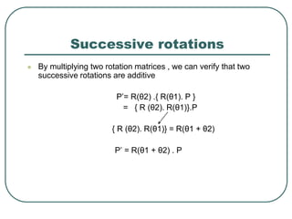
Successive translations are additive
P’= T(tx1, ty1) .[T(tx2, ty2)] P
= {T(tx1, ty1). T(tx2, ty2)}.P
T(tx1, ty1). T(tx2, ty2) = T(tx1+tx2 , ty1 + ty2)
1 0 tx1+tx2
0 1 ty1+ty2
0 0 1
1 0 tx1
0 1 ty1
0 0 1
1 0 tx2
0 1 ty2
0 0 1
=

21. Successive rotations
 By multiplying two rotation matrices , we can verify that two
successive rotations are additive
P’= R(θ2) .{ R(θ1). P }
= { R (θ2). R(θ1)}.P
{ R (θ2). R(θ1)} = R(θ1 + θ2)
P’ = R(θ1 + θ2) . P

22. Successive Scaling operations
Sx1.sx2 0 0
0 sy1sy2 0
0 0 1
sx1 0 0
0 sy1 0
0 0 1
sx2 0 0
0 sy2 0
0 0 1
=
S(sx2,sy2).S(sx1,sy1) = S(sx1.sx2 , sy1,sy2)
The resulting matrix in this case indicates that successive scaling
operations are multiplicative

23. General pivot point rotation
 With a graphics package that only provides a rotate
function for revolving objects about the coordinate origin,
we can generate rotations about any selected pivot point
(x, y,) by performing sequence of translate-rotate translate
operations.

24. General pivot point rotation
 Translate the object so that pivot-position is moved to the
coordinate origin
 Rotate the object about the coordinate origin
 Translate the object so that the pivot point is returned to its original
position
(xr,yr)
(a)
Original Position
of Object and
pivot point
(b)
Translation of
object so that
pivot point
(xr,yr)is at origin
(c)
Rotation was
about origin
(d)
Translation of the object
so that the pivot point is
returned to position
(xr,yr)

25. General pivot point rotation
1 0 xr
0 1 yr
0 0 1
cosθ -sinθ 0
sinθ cosθ 0
0 0 1
1 0 -xr
0 1 -yr
0 0 1
=
cosθ -sinθ xr(1- cosθ)+ yr sinθ
sinθ cosθ yr(1- cosθ) - xr sinθ
0 0 1
Can also be expressed as T(xr,yr).R(θ).T(-xr,-yr) = R(xr,yr,θ)

26. General fixed point scaling
 Translate object so that the fixed point coincides with the
coordinate origin
 Scale the object with respect to the coordinate origin
 Use the inverse translation of step 1 to return the object to its
original position
(xf,yf)
(a)
Original Position
of Object and
Fixed point
(b)
Translation of
object so that
fixed point
(xf,yf)is at origin
(c)
scaling was
about origin
(d)
Translation of the object
so that the Fixed point
is returned to position
(xf,yf)

27. General fixed point Scaling
1 0 xf
0 1 yf
0 0 1
sx 0 0
0 sy 0
0 0 1
1 0 -xf
0 1 -yf
0 0 1
=
sx 0 xf(1- sx)
0 sy yf(1- sy)
0 0 1
Can also be expressed as T(xf,yf).S(sx,sy).T(-xf,-yf) = S(xf, yf, sx, sy)

30. Transformations Properties
 Concatenation properties
A.B.C = (A.B).C = A.(B.C)
Matrix products can be evaluated from left to right or from right
to left
 However they are not commutative
A.B ≠ B.A
 Hence one must be careful in order that the composite
transformation matrix is evaluated

31. Matrix Composition
 Be aware: order of transformations
matters
• Matrix multiplication is not commutative
p’ = T * R * S * p
“Global” “Local”

32. Order of Transformations
 Reversing the order in which a sequence of transformations is
performed may effect the transformed position of an object.
 In (a) object is first translated , then rotated
 In (b) the object is rotated first and then translated
(a) (b)

33. General Composite
transformations
 A general 2D transformation representing a combination of translations,
rotations and scalings are expressed as,
 rsij represent multiplicative rotation-scaling terms , trsx and trsy are the
translational terms containing combinations of translations and scaling
parameters
X’
Y’
1
=
rsxx rsxy trsx
rsyx rsyy trsy
0 0 1
X
Y
1

34. Composite transformations
 For example , if an object is to be scaled and rotated about its
center coordinates (xc,yc) and then translated , the composite
transformation matrix looks like
 T(tx,ty). R(xc,yc,θ) . S(xc, yc, sx, sy)
=
sxcosθ -sysinθ xc(1-sxcosθ) + yc sy sinθ +tx
sxsin θ sycos θ yc(1-sycosθ) – xc sx sinθ + ty
0 0 1
Represents 9 multiplications and 6 additions

35. Composite Transformations
 The explicit calculation has only 4 multiplications and 4
additions
x’ = x.rsxx + y.r sxy + tr sx
y’ = x. rsyx + y. rsyy + tr sy
 The efficient implementation is to
• Formulate transformation matrices
• Concatenate transformation sequence
• Calculate transformed coordinates using the explicit
equation shown above

36. A general rigid body
transformation matrix
 A general rigid body transformation involving only translations
and rotations can be expressed in the form
rxx rxy trx
ryx ryy try
0 0 1

37. Other transformations
 Reflection is a transformation that produces a mirror image
of an object. It is obtained by rotating the object by 180 deg
about the reflection axis
1
2 3
3’2’
1’
Original position
Reflected position
Reflection about the line y=0, the
axis , is accomplished with the
transformation matrix
1 0 0
0 -1 0
0 0 1

38. Reflection
-1 0 0
0 1 0
0 0 11’
3’
2’
3
2
1
Original position Reflected position

39. Reflection
-1 0 0
0 -1 0
0 0 1
1’
2’
3’
3
2
1
Original position
Reflected position
Reflection of an object
relative to an axis
perpendicular to the xy plane
and passing through the
coordinate origin

40. Reflection of an object w.r.t the
line y=x
0 1 0
1 0 0
0 0 1
1’
3’
2’
3
2 1
Original position
Reflected position

41. Shear Transformations
 Shear is a transformation that distorts the shape of an
object such that the transformed shape appears as if the object
were composed of internal layers that had been caused to slide
over each other
 Two common shearing transformations are those that shift
coordinate x values and those that shift y values
 An x direction shear relative to the x axis is produced with the
transformation matrix
1 shx 0
0 1 0
0 0 1
Which transforms coordinate positions as
X’ = x + shx.y y’ =y

42. Shear tranformations
Yref =-1
Yref =-1
(0,1) (1,1)
(1,0)(0,0)
(1,1) (2,1)
(3/2,0)(1/2,0)
We can generate x-direction shears relative to other referance lines with
1 shx -shx yref
0 1 0
0 0 1
With coordinate positions transformed as
X’= x + shx (y - yref) y’ = y

43. Shear transformation
A y-direction shear relative to the line x = xref is generated with the
transformation matrix
1 0 0
Shy 1 -shy.xref
0 0 1
This generates transformed coordinate
positions
X’ = x y’ = shy (x – xref) + y
(1,1)(0,1)
(0,0) (1,0)
(1,2)
(1,1)
(0,1/2)
(0,3/2)
Xref = -1

44. Affine Transformations
 Affine transformations are combinations of …
• Linear transformations, and
• Translations
 Properties of affine transformations:
• Origin does not necessarily map to origin
• Lines map to lines
• Parallel lines remain parallel after transformation
• X=axxx+axyy=bx
• Y=ayxx+ayyy+by

























w
y
x
fed
cba
w
y
x
100
'
'