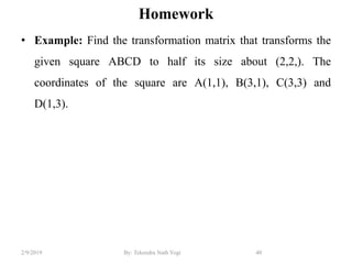
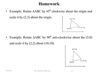
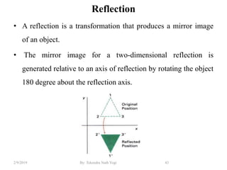
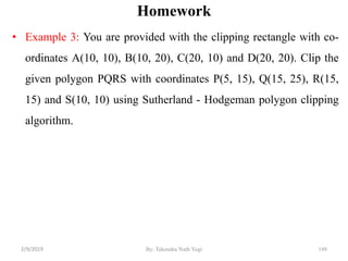
Downloaded 303 times
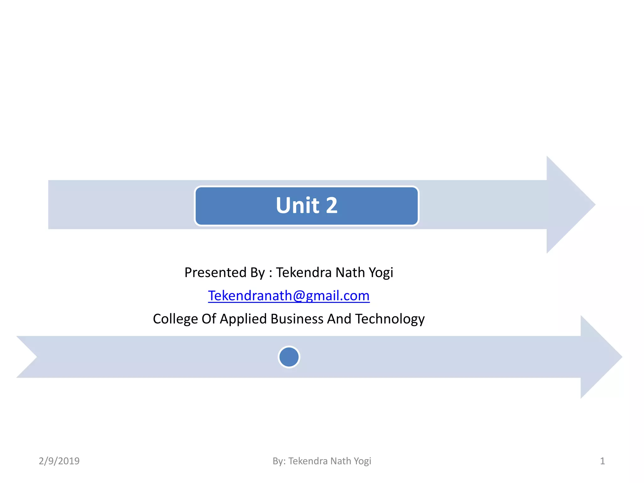
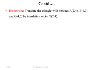
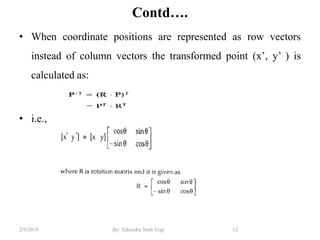
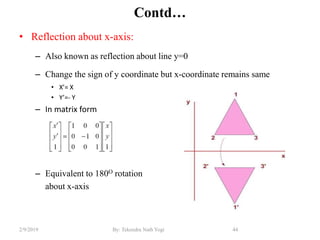

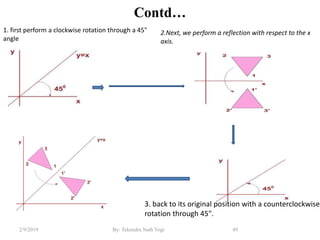

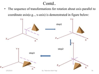
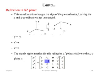
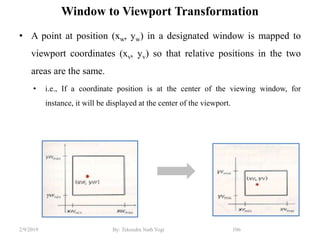
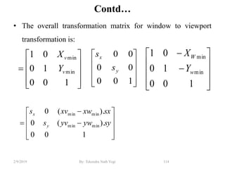
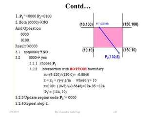
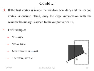
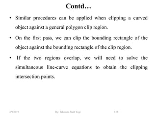
![Contd…
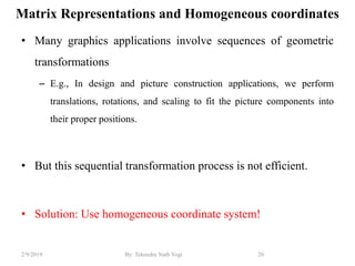
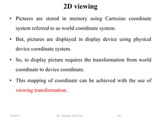
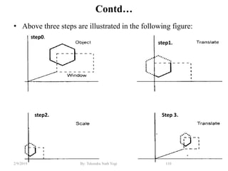
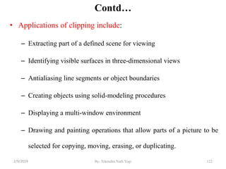
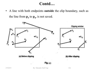
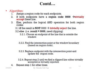
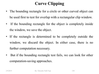
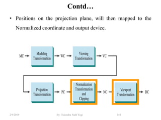
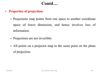
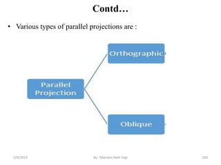
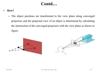
• Every end-point is labelled with the appropriate region code
• For example:
wymax
wymin
wxmin wxmax
Window
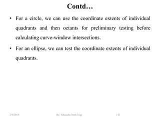
P3 [0001]
P6 [0000]
P5 [0000]
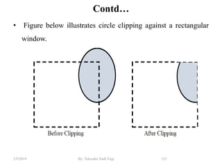
P7 [0001]
P10 [0100]
P9 [0000]
P4 [1000]
P8 [0010]
P12 [0010]
P11 [1010]
P13 [0101] P14 [0110]
129By: Tekendra Nath Yogi2/9/2019](https://image.slidesharecdn.com/unit2-190209042007/85/B-SC-CSIT-Computer-Graphics-Unit-2-By-Tekendra-Nath-Yogi-129-320.jpg)
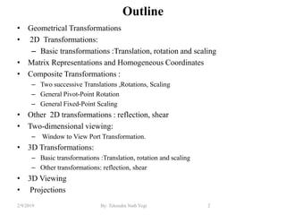
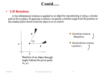
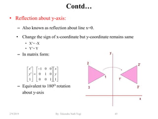
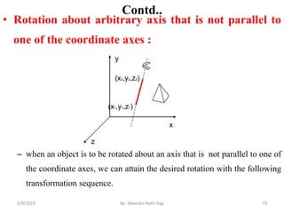
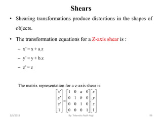
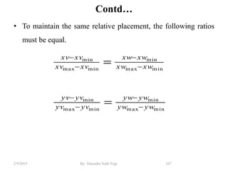
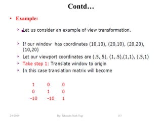
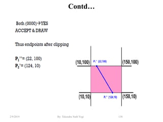
![Contd…
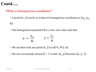
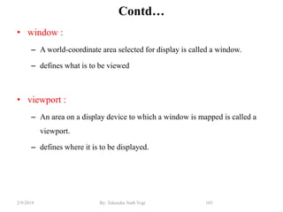
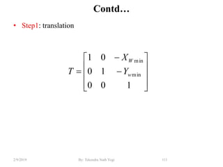
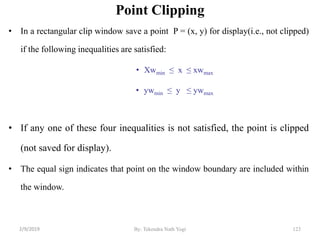
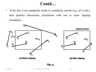
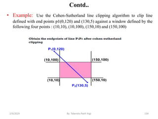
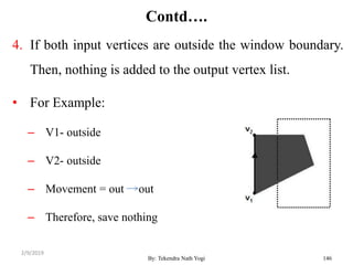
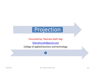
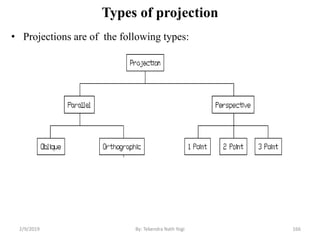
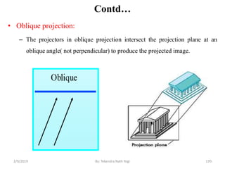
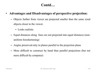
• Step2: Trivial acceptance of line segment
– Lines completely contained within the window boundaries have region code
[0000] for both end-points so are not clipped. i.e., accept these lines
trivially.
– E.g., line p5p6
wymax
wymin
wxmin wxmax
Window
P3 [0001]
P6 [0000]
P5 [0000]
P7 [0001]
P10 [0100]
P9 [0000]
P4 [1000]
P8 [0010]
P12 [0010]
P11 [1010]
P13 [0101] P14 [0110]
130By: Tekendra Nath Yogi2/9/2019](https://image.slidesharecdn.com/unit2-190209042007/85/B-SC-CSIT-Computer-Graphics-Unit-2-By-Tekendra-Nath-Yogi-130-320.jpg)
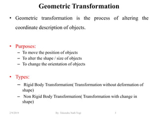
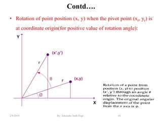
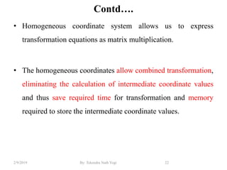
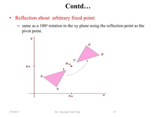
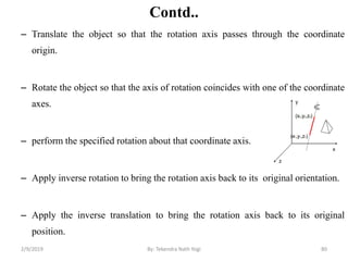
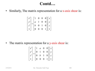
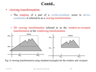
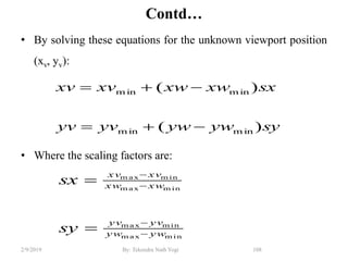
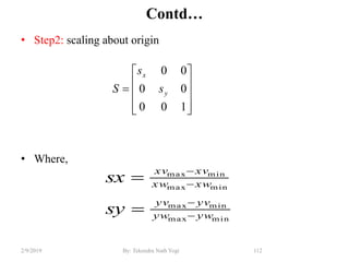
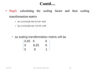
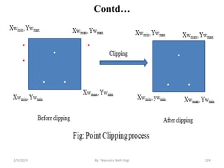
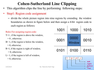
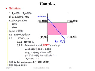
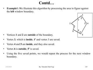
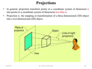
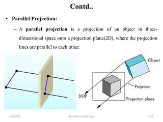
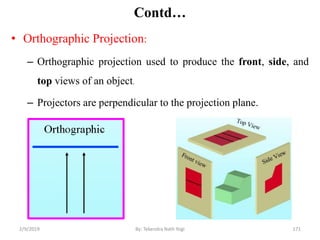
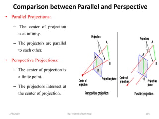
![• Step3: Trivial rejection and clipping
– 3.1 : Any lines that have a 1 in the same bit position in the
region-codes for each endpoint are completely outside and we
reject these lines.
– The AND operation can efficiently check this: If the logical AND of both
region codes result is not 0000, the line is completely outside the
clipping region so clipped.
Contd…
wymax
wymin
wxmin wxmax
Window
P3 [0001]
P6 [0000]
P5 [0000]
P7 [0001]
P10 [0100]
P9 [0000]
P4 [1000]
P8 [0010]
P12 [0010]
P11 [1010]
P13 [0101] P14 [0110]
131By: Tekendra Nath Yogi2/9/2019](https://image.slidesharecdn.com/unit2-190209042007/85/B-SC-CSIT-Computer-Graphics-Unit-2-By-Tekendra-Nath-Yogi-131-320.jpg)
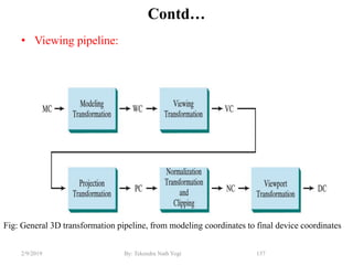


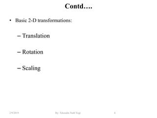
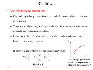
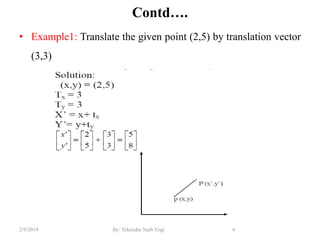
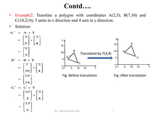
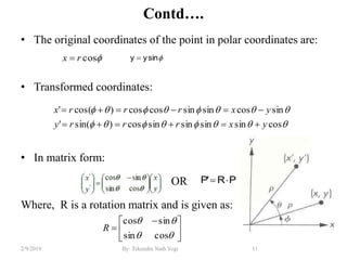
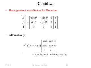
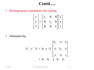
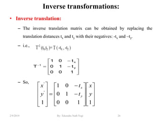
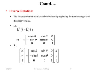
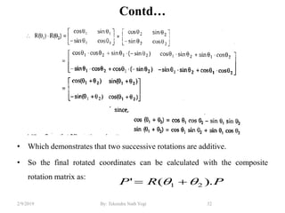
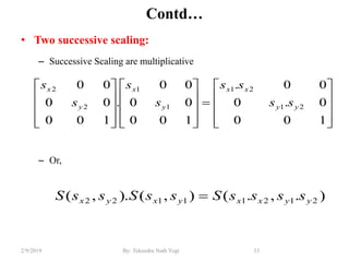
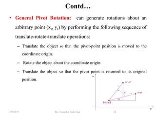
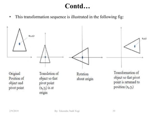
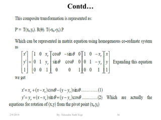
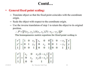
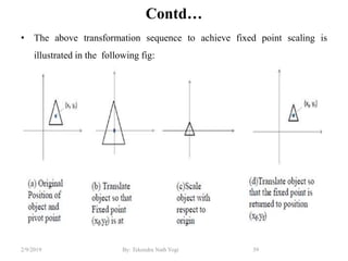
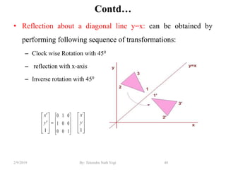
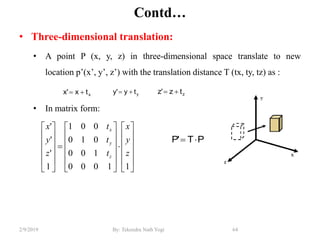
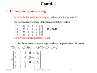
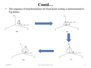
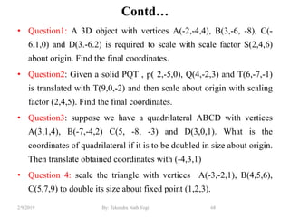
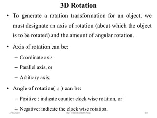
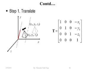
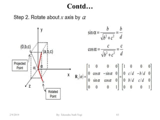
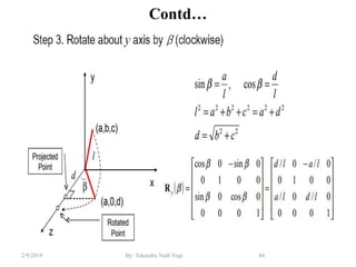
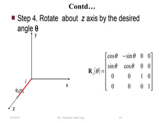
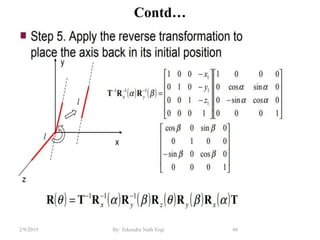
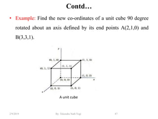
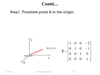
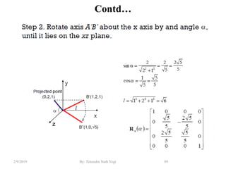
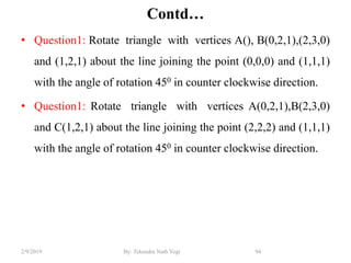
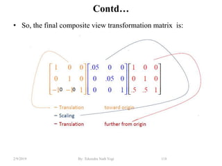
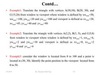
The document discusses various 2D and 3D geometric transformations including translation, rotation, scaling, and their implementations using matrix representations and homogeneous coordinates. It provides examples of translating, rotating, and scaling points and polygons. It also covers composite transformations, inverse transformations, and applications to 2D and 3D viewing. Homework examples are provided to practice applying the different transformation types.