This document provides an introduction and overview of ordinary differential equations (ODEs) for engineers. It defines key concepts such as ODEs, solutions, order of an ODE, linear and homogeneous equations. It also discusses systems of ODEs and approaches for finding solutions, including analytical and numerical methods. The document serves as notes for an engineering course on ODEs, covering topics like first order, nth order, and systems of linear and nonlinear differential equations.


![Contents vii
3. N-TH ORDER DIFFERENTIAL EQUATIONS 25
1 Introduction 25
2 (*)Fundamental Theorem of Existence and Uniqueness 26
2.1 Theorem of Existence and Uniqueness (I) 26
2.2 Theorem of Existence and Uniqueness (II) 27
2.3 Theorem of Existence and Uniqueness (III) 27
3 Linear Equations 27
3.1 Basic Concepts and General Properties 27
3.1.1 Linearity 28
3.1.2 Superposition of Solutions 29
3.1.3 (∗) Kernel of Linear operator L(y) 29
3.2 New Notations 29
4 Basic Theory of Linear Differential Equations 30
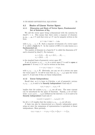
4.1 Basics of Linear Vector Space 31
4.1.1 Dimension and Basis of Vector Space, Fundamental
Set of Solutions of Eq. 31
4.1.2 Linear Independency 31
4.2 Wronskian of n-functions 34
4.2.1 Definition 34
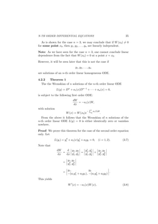
4.2.2 Theorem 1 35
4.2.3 Theorem 2 36
4.2.4 The Solutions of L[y] = 0 as a Linear Vector Space 38
5 Finding the Solutions in terms of the Method with Differential
Operators 38
5.1 Solutions for Equations with Constants Coefficients
38
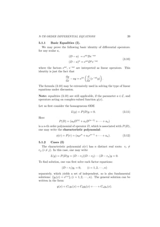
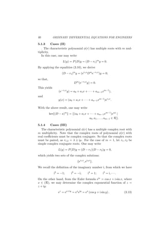
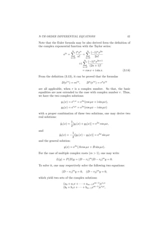
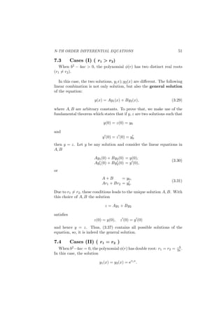
5.1.1 Basic Equalities (I). 39
5.1.2 Cases (I) 39
5.1.3 Cases (II) 40
5.1.4 Cases (III) 40
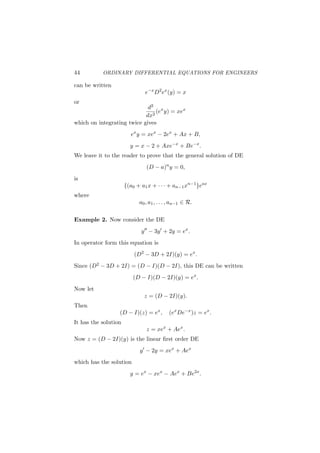
5.1.5 Summary 42
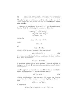
5.1.6 Theorem 1 43
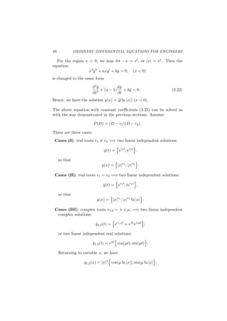
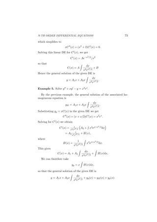
6 Solutions for Equations with Variable Coefficients 46
6.1 Euler Equations 47
7 Finding the Solutions in terms of the Method with Undetermined
Parameters 49
7.1 Solutions for Equations with Constants Coefficients
50
7.2 Basic Equalities (II) 50](https://image.slidesharecdn.com/ode-220514071737-88715c85/85/ODE-pdf-6-320.jpg)


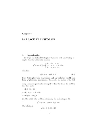
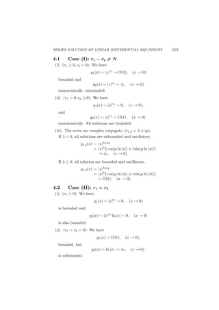
![Chapter 1
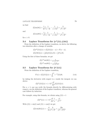
INTRODUCTION
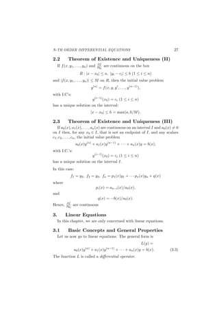
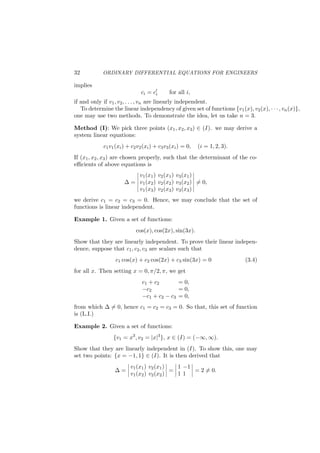
1. Definitions and Basic Concepts
1.1 Ordinary Differential Equation (ODE)
An equation involving the derivatives of an unknown function y of a
single variable x over an interval x ∈ (I). More clearly and precisely
speaking, a well defined ODE must the following features:
It can be written in the form:
F[x, y, y′
, y′′
, · · · , yn
] = 0; (1.1)
where the mathematical expression on the right hand side contains
(1). variable x, (2). function y of x, and (3). some derivatives of y
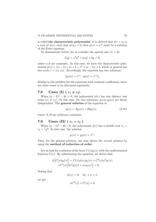
with respect to x;
The values of variables x, y must be specified in a certain number
field, such as N, R, or C;
The variation region of variable x of Eq. must be specified, such as
x ∈ (I) = (a, b).
1.2 Solution
Any function y = f(x) which satisfies this equation over the interval
(I) is called a solution of the ODE. More clearly speaking, function ϕ(x)
is called a solution of the give EQ. (1.1), if the following requirements
are satisfies:
The function ϕ(x) is defined in the region x ∈ (I);
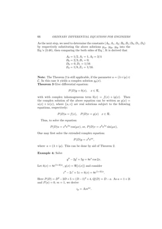
The function ϕ(x) is differentiable, hence, {ϕ′(x), · · · , ϕ(n)(x)} all
exit, in the region x ∈ (I);
1](https://image.slidesharecdn.com/ode-220514071737-88715c85/85/ODE-pdf-12-320.jpg)
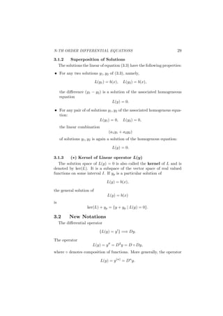
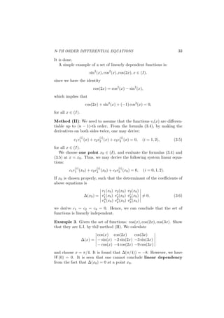
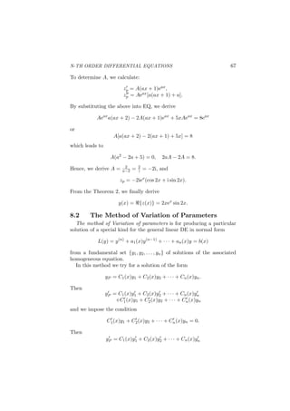
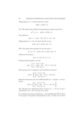
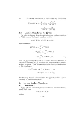
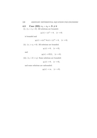
![2 ORDINARY DIFFERENTIAL EQUATIONS FOR ENGINEERS
With the replacements of the variables y, y′, · · · , y(n) in 1.1 by the
functions ϕ(x), ϕ′(x), · · · , ϕ(n)(x), the EQ. (1.1) becomes an identity
over x ∈ (I). In other words, the right hand side of Eq. (1.1) becomes
to zero for all x ∈ (I).
For example, one can verify that y = e2x is a solution of the ODE
y′
= 2y, x ∈ (−∞, ∞),
and y = sin(x2) is a solution of the ODE
xy′′
− y′
+ 4x3
y = 0, x ∈ (−∞, ∞).
1.3 Order n of the DE
An ODE is said to be order n, if y(n) is the highest order derivative
occurring in the equation. The simplest first order ODE is y′ = g(x).
Note that the expression F on the right hand side of an n-th order
ODE: F[x, y, y′, . . . , y(n)] = 0 can be considered as a function of n + 2
variables (x, u0, u1, . . . , un). Namely, one may write
F(x, u0, u1, · · · , un) = 0.
Thus, the equations
xy′′
+ y = x3
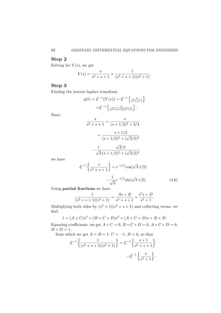
, y′
+ y2
= 0, y′′′
+ 2y′
+ y = 0
which are examples of ODE’s of second order, first order and third order
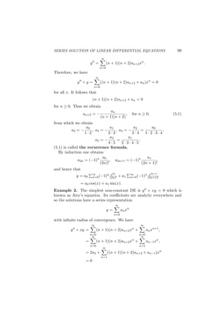
respectively, can be in the forms:
F(x, u0, u1, u2) = xu2 + u0 − x3,
F(x, u0, u1) = u1 + u2
0,
F(x, u0, u1, u2, u3) = u3 + 2u1 + u0.
respectively.
1.4 Linear Equation:
If the function F is linear in the variables u0, u1, . . . , un, which means
every term in F is proportional to u0, u1, . . . , un, the ODE is said to be
linear. If, in addition, F is homogeneous then the ODE is said to be
homogeneous. The first of the above examples above is linear are linear,
the second is non-linear and the third is linear and homogeneous. The
general n-th order linear ODE can be written
an(x)dny
dxn + an−1(x)dn−1y
dxn−1 + · · · + a1(x)dy
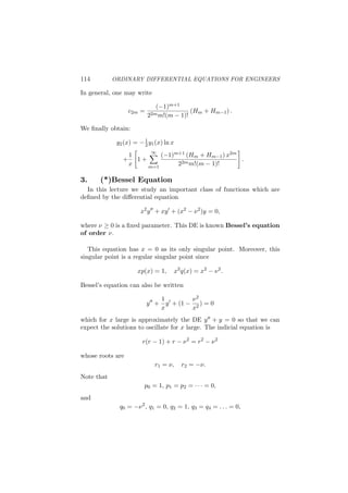
dx
+a0(x)y = b(x).](https://image.slidesharecdn.com/ode-220514071737-88715c85/85/ODE-pdf-13-320.jpg)
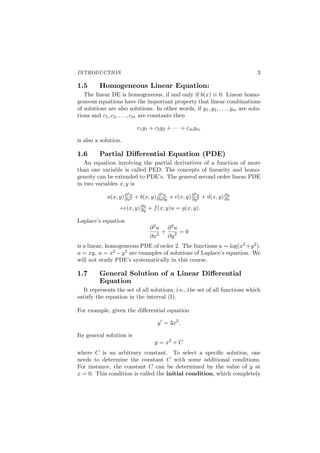

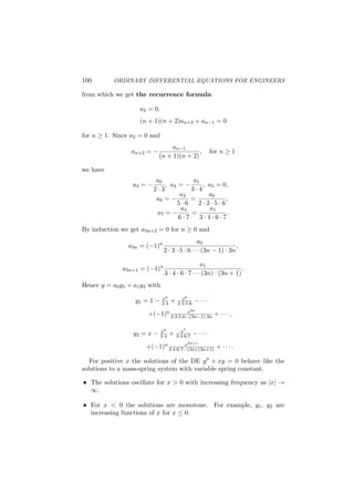
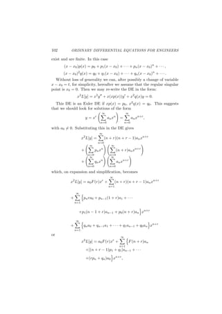
![8 ORDINARY DIFFERENTIAL EQUATIONS FOR ENGINEERS
1.1 Linear homogeneous equation
Let us first consider the simple case: q(x) = 0, namely,
dy
dx
+ p(x)y = 0. (2.1)
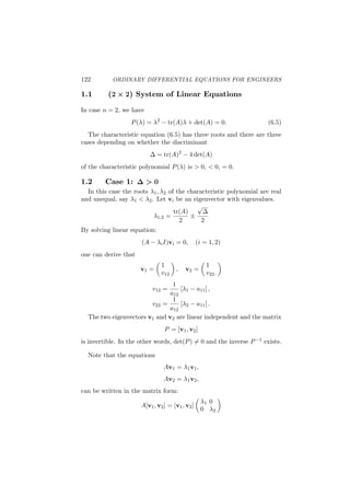
To find the solutions, we proceed in the following three steps:
Assume that the solution exists and in the form y = y(x);
Find the necessary form of the function y(x). In doing so, by the
definition of the solution, one substitute the function y(x) in the Eq.,
and try to transform the EQ. in such a way that its LHS of EQ. is a
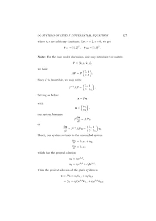
complete differentiation d
dx[.....], while its RHS is a known function.
Verify y(x) is indeed a solution.
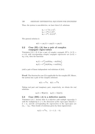
In the step #2, with the chain law of derivative, one may transform Eq.
(2.1) into the following form:
y′(x)
y
=
d
dx
ln |y(x)| = −p(x).
Its LHS is now changed a complete differentiation with respect to x,
while its RHS is a known function. By integrating both sides, we derive
ln |y(x)| = −
∫
p(x)dx + C,
or
y = ±C1e−
∫
p(x)dx
,
where C, as well as C1 = eC > 0, is arbitrary constant. As C=0, y(x) = 0
is a trivial solution, we derive the necessary form of solution:
y = Ae−
∫
p(x)dx
. (2.2)
As the final step of derivation, one can verify the function (2.2) is indeed
a solution for any value of constant A. In summary, we deduce that (2.2)
is the form of solution, that contains all possible solution. Hence, one
can call (2.2) as the general solution of Eq. (2.1).
1.2 Linear inhomogeneous equation
We now consider the general case:
dy
dx
+ p(x)y = q(x).](https://image.slidesharecdn.com/ode-220514071737-88715c85/85/ODE-pdf-19-320.jpg)
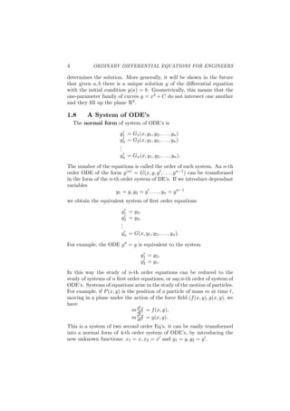
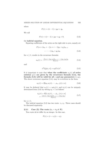
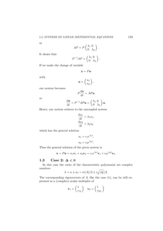
![FIRST ORDER DIFFERENTIAL EQUATIONS 9
We still proceed in the three steps as we did in the previous subsection.
However, now in the step #2 one cannot directly transform the LHS of
Eq. in the complete differential form as we did for the case of homoge-
neous Eq. For this purpose, we multiply the both sides of our differential
equation with a factor µ(x) ̸= 0. Then our equation is equivalent (has
the same solutions) to the equation
µ(x)y′
(x) + µ(x)p(x)y(x) = µ(x)q(x).
We wish that with a properly chosen function µ(x),
µ(x)y′
(x) + µ(x)p(x)y(x) =
d
dx
[µ(x)y(x)].
For this purpose, the function µ(x) must has the property
µ′
(x) = p(x)µ(x), (2.3)
and µ(x) ̸= 0 for all x. By solving the linear homogeneous equation
(2.3), one obtain
µ(x) = e
∫
p(x)dx
. (2.4)
With this function, which is called an integrating factor, our equation
is now transformed into the form that we wanted:
d
dx
[µ(x)y(x)] = µ(x)q(x), (2.5)
Integrating both sides, we get
µ(x)y =
∫
µ(x)q(x)dx + C
with C an arbitrary constant. Solving for y, we get
y =
1
µ(x)
∫
µ(x)q(x)dx +
C
µ(x)
= yP (x) + yH(x) (2.6)
as the general solution for the general linear first order ODE
y′
+ p(x)y = q(x).
In solution (2.6):
the first part, yP (x): a particular solution of the inhomogeneous
equation,](https://image.slidesharecdn.com/ode-220514071737-88715c85/85/ODE-pdf-20-320.jpg)
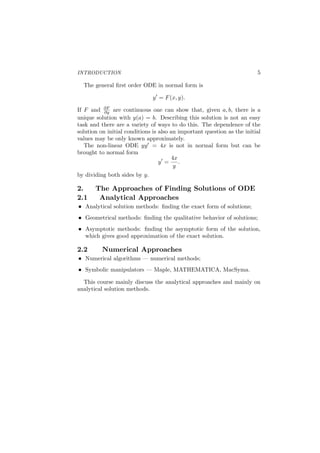
![12 ORDINARY DIFFERENTIAL EQUATIONS FOR ENGINEERS
We apply the procedure of three steps for the solutions as before. Assume
that the solution y = y(x) exists, and h(y) ̸= 0 as x ∈ (I). Then by
dividing both sides by h[y(x)], it becomes
y′(x)
h[y(x)]
= g(x). (2.8)
Of course this is not valid for those solutions y = y(x) at the points
where h[y(x)] = 0. Furthermore, we assume that the LHS can be written
in the form of complete differentiation: d
dxH[y(x)], where H[y(x)] is a
composite function of x to be determined. Once we find the function
H(y), we may write
H[y(x)] =
∫
y′(x)
h[y(x)]
dx =
∫
g(x)dx + C.
However, by chain rule we have
d
dx
H[y(x)] = H′
(y)y′
(x).
By comparing the above with the LHS of (3.33), it follows that
H′
(y) =
1
h(y)
.
Thus, we derive that
H(y) =
∫
dy
h(y)
=
∫
g(x)dx + C, (2.9)
This gives the implicit form of the solution. It determines the value of y
implicitly in terms of x. The function given in (2.9) can be easily verified
as indeed a solution. Note that with the assumption h(y) ̸= 0 at the
beginning of the derivation, some solution may be excluded in (2.9). As
a matter of fact, one can verify that the Eq. may allow the constant
solutions,
y = y∗, (2.10)
as h(y∗) = 0.
Example 1: y′ = x−5
y2 .
To solve it using the above method we multiply both sides of the
equation by y2 to get
y2
y′
= (x − 5).](https://image.slidesharecdn.com/ode-220514071737-88715c85/85/ODE-pdf-23-320.jpg)
![FIRST ORDER DIFFERENTIAL EQUATIONS 13
Integrating both sides we get y3/3 = x2/2 − 5x + C. Hence,
y =
[
3x2
/2 − 15x + C1
]1/3
.
Example 2: y′ = y−1
x+3 (x > −3). By inspection, y = 1 is a solution.
Dividing both sides of the given DE by y − 1 we get
y′
y − 1
=
1
x + 3
.
This will be possible for those x where y(x) ̸= 1. Integrating both sides
we get ∫
y′
y − 1
dx =
∫
dx
x + 3
+ C1,
from which we get ln |y − 1| = ln(x + 3) + C1. Thus |y − 1| = eC1 (x + 3)
from which y − 1 = ±eC1 (x + 3). If we let C = ±eC1 , we get
y = 1 + C(x + 3)
. Since y = 1 was found to be a solution by inspection the general
solution is
y = 1 + C(x + 3),
where C can be any scalar. For any (a, b) with a ̸= −3, there is only one
member of this family which passes through (a, b).
However, it is seen that there is a family of lines passing through
(−3, 1), while no solution line passing through (−3, b) with b ̸= 1). Here,
x = −3 is a singular point.
Example 3: y′ = y cos x
1+2y2 . Transforming in the standard form then
integrating both sides we get
∫
(1 + 2y2)
y
dy =
∫
cos x dx + C,
from which we get a family of the solutions:
ln |y| + y2
= sin x + C,
where C is an arbitrary constant. However, this is not the general solu-
tion of the equation, as it does not contains, for instance, the solution:
y = 0. With I.C.: y(0)=1, we get C = 1, hence, the solution:
ln |y| + y2
= sin x + 1.](https://image.slidesharecdn.com/ode-220514071737-88715c85/85/ODE-pdf-24-320.jpg)
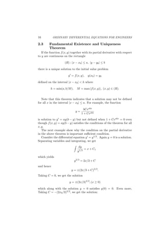

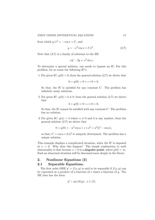
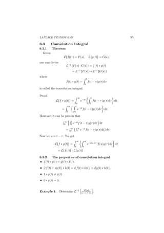
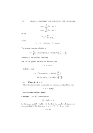
![FIRST ORDER DIFFERENTIAL EQUATIONS 17
y =
{
0 (0 ≤ x ≤ x0)
±[2(x − x0)/3]3/2
, (x ≥ x0)
which also satisfies y(0) = 0. So the initial value problem
y′
= y1/3
, y(0) = 0
does not have a unique solution. The reason this is so is due to the fact
that
∂f
∂y
(x, y) =
1
3y2/3
is not continuous when y = 0.
Many differential equations become linear or separable after a change
of variable. We now give two examples of this.
2.4 Bernoulli Equation:
y′
= p(x)y + q(x)yn
(n ̸= 1).
Note that y = 0 is a solution. To solve this equation, we set
u = yα
,
where α is to be determined. Then, we have
u′
= αyα−1
y′
,
hence, our differential equation becomes
u′
/α = p(x)u + q(x)yα+n−1
. (2.11)
Now set
α = 1 − n,
Thus, (2.11) is reduced to
u′
/α = p(x)u + q(x), (2.12)
which is linear. We know how to solve this for u from which we get solve
u = y1−n
to get
y = u1/(1−n)
. (2.13)](https://image.slidesharecdn.com/ode-220514071737-88715c85/85/ODE-pdf-36-320.jpg)
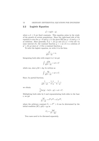
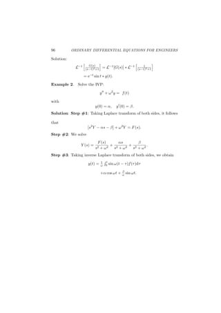
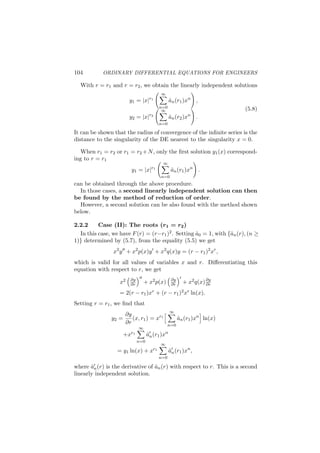
![20 ORDINARY DIFFERENTIAL EQUATIONS FOR ENGINEERS
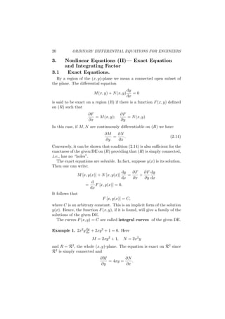
3. Nonlinear Equations (II)— Exact Equation
and Integrating Factor
3.1 Exact Equations.
By a region of the (x, y)-plane we mean a connected open subset of
the plane. The differential equation
M(x, y) + N(x, y)
dy
dx
= 0
is said to be exact on a region (R) if there is a function F(x, y) defined
on (R) such that
∂F
∂x
= M(x, y);
∂F
∂y
= N(x, y)
In this case, if M, N are continuously differentiable on (R) we have
∂M
∂y
=
∂N
∂x
. (2.14)
Conversely, it can be shown that condition (2.14) is also sufficient for the
exactness of the given DE on (R) providing that (R) is simply connected,
.i.e., has no “holes”.
The exact equations are solvable. In fact, suppose y(x) is its solution.
Then one can write:
M [x, y(x)] + N [x, y(x)]
dy
dx
=
∂F
∂x
+
∂F
∂y
dy
dx
=
d
dx
F [x, y(x)] = 0.
It follows that
F [x, y(x)] = C,
where C is an arbitrary constant. This is an implicit form of the solution
y(x). Hence, the function F(x, y), if it is found, will give a family of the
solutions of the given DE.
The curves F(x, y) = C are called integral curves of the given DE.
Example 1. 2x2y dy
dx + 2xy2 + 1 = 0. Here
M = 2xy2
+ 1, N = 2x2
y
and R = R2, the whole (x, y)-plane. The equation is exact on R2 since
R2 is simply connected and
∂M
∂y
= 4xy =
∂N
∂x
.](https://image.slidesharecdn.com/ode-220514071737-88715c85/85/ODE-pdf-39-320.jpg)
![28 ORDINARY DIFFERENTIAL EQUATIONS FOR ENGINEERS
3.1.1 Linearity
The characteristic features of linear operator L is that
With any constants (C1, C2),
L(C1y1 + C2y2) = C1L(y1) + C2L(y2).
With any given functions of x, p1(x), p2(x), and the Linear operators,
L1(y) = a0(x)y(n)
+ a1(x)y(n−1)
+ · · · + an(x)y
L2(y) = b0(x)y(n)
+ b1(x)y(n−1)
+ · · · + bn(x)y,
the function
p1L1 + p2L2
defined by
(p1L1 + p2L2)(y) = p1(x)L1(y) + p2(x)L2(y)
=
[
p(x)a0(x) + p2(x)b0(x)
]
y(n) + · · ·
+ [p1(x)an(x) + p2(x)bn(x)] y
is again a linear differential operator.
Linear operators in general are subject to the distributive law:
L(L1 + L2) = LL1 + LL2,
(L1 + L2)L = L1L + L2L.
Linear operators with constant coefficients are commutative:
L1L2 = L2L1.
Note: In general the linear operators with non-constant coeffi-
cients are not commutative: Namely,
L1L2 ̸= L2L1.
For instance, let L1 = a(x) d
dx , L2 = d
dx.
L1L2 = a(x)
d2
dx2
̸= L2L1 =
d
dx
[
a(x)
d
dx
]
.](https://image.slidesharecdn.com/ode-220514071737-88715c85/85/ODE-pdf-71-320.jpg)
![30 ORDINARY DIFFERENTIAL EQUATIONS FOR ENGINEERS
The identity operator I is defined by
I(y) = y = D0
y.
By definition D0 = I. The general linear n-th order ODE can therefore
be written
[
a0(x)Dn
+ a1(x)Dn−1
+ · · · + an(x)I
]
(y) = b(x).
4. Basic Theory of Linear Differential
Equations
In this section we will develop the theory of linear differential equa-
tions. The starting point is the fundamental existence theorem for the
general n-th order ODE L(y) = b(x), where
L(y) = Dn
+ a1(x)Dn−1
+ · · · + an(x).
We will also assume that a0(x) ̸= 0, a1(x), . . . , an(x), b(x) are continuous
functions on the interval I.
The fundamental theory says that for any x0 ∈ I, the initial value
problem
L(y) = b(x)
with the initial conditions:
y(x0) = d1, y′
(x0) = d2, . . . , y(n−1)
(x0) = dn
has a unique solution y = y(x) for any (d1, d2, . . . , dn) ∈ Rn.
From the above, one may deduce that the general solution of n-th
order linear equation contains n arbitrary constants. It can be also
deduced that the above solution can be expressed in the form:
y(x) = d1y1(x) + · · · + dnyn(x),
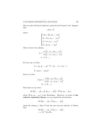
where the {yi(x)}, (i = 1, 2, · · · , n) is the set of the solutions for the IVP
with IC’s: {
y(i−1)(x0) = 1, i = 1, 2, · · · n)
y(k−1)(x0) = 0, (k ̸= i, 1 ≤ k ≤ n).
In general, if the equation L(y) = 0 has a set of n solutions: {y1(x), · · · yn(x)}
of the equation, such that any solution y(x) of the equation can be ex-
pressed in the form:
y(x) = c1y1(x) + · · · + cnyn(x),
with a proper set of constants {c1, · · · , cn}, then the solutions {yi(x), i =
1, 2, · · · , n} is called a set of fundamental solutions of the equation.](https://image.slidesharecdn.com/ode-220514071737-88715c85/85/ODE-pdf-73-320.jpg)

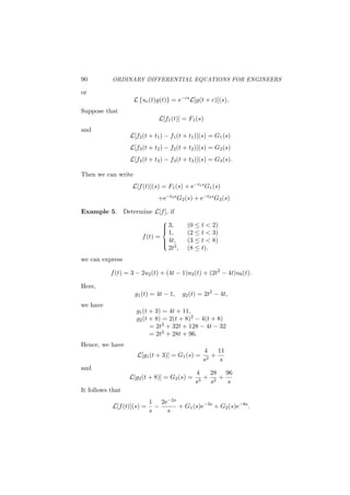
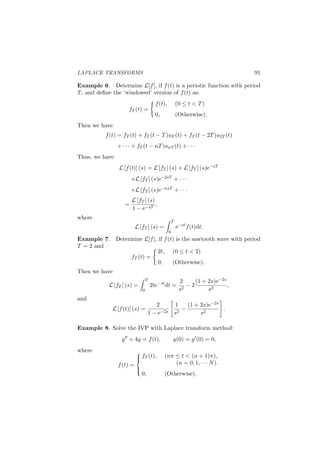
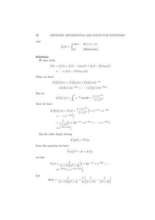


![Week 6 [compatibility mode]](https://cdn.slidesharecdn.com/ss_thumbnails/week6compatibilitymode-130213163919-phpapp02-thumbnail.jpg?width=640&height=640&fit=bounds)


