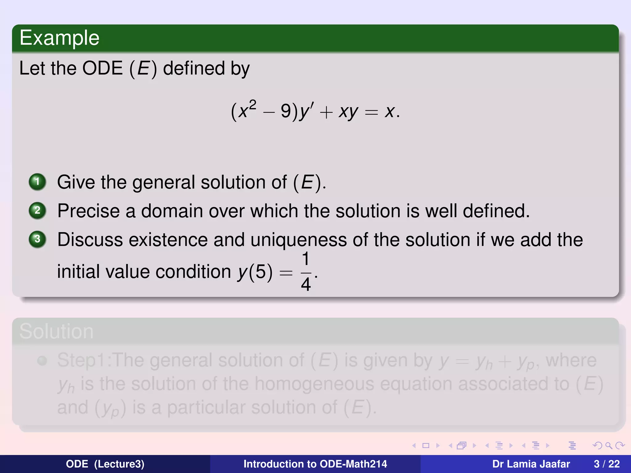
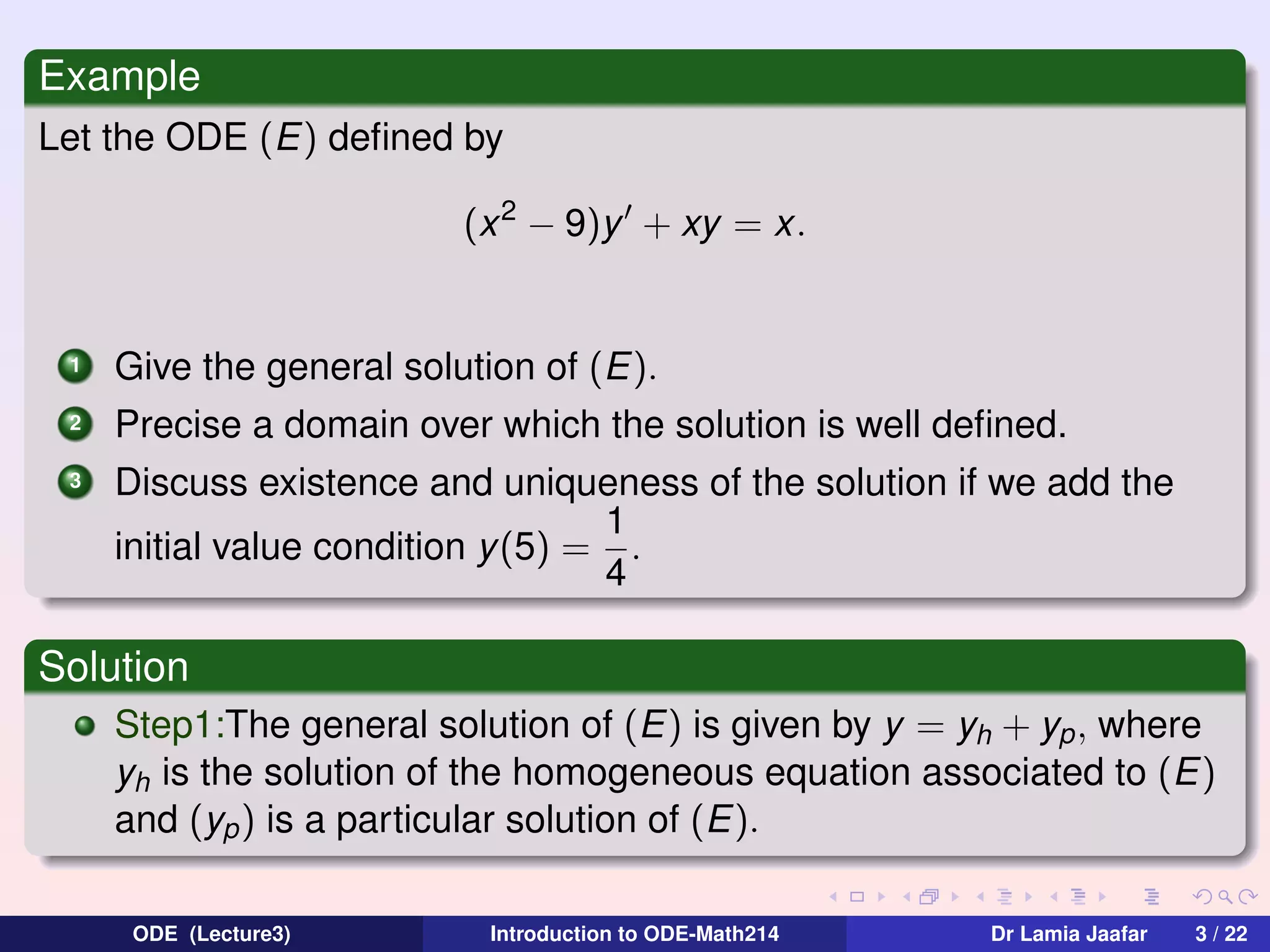
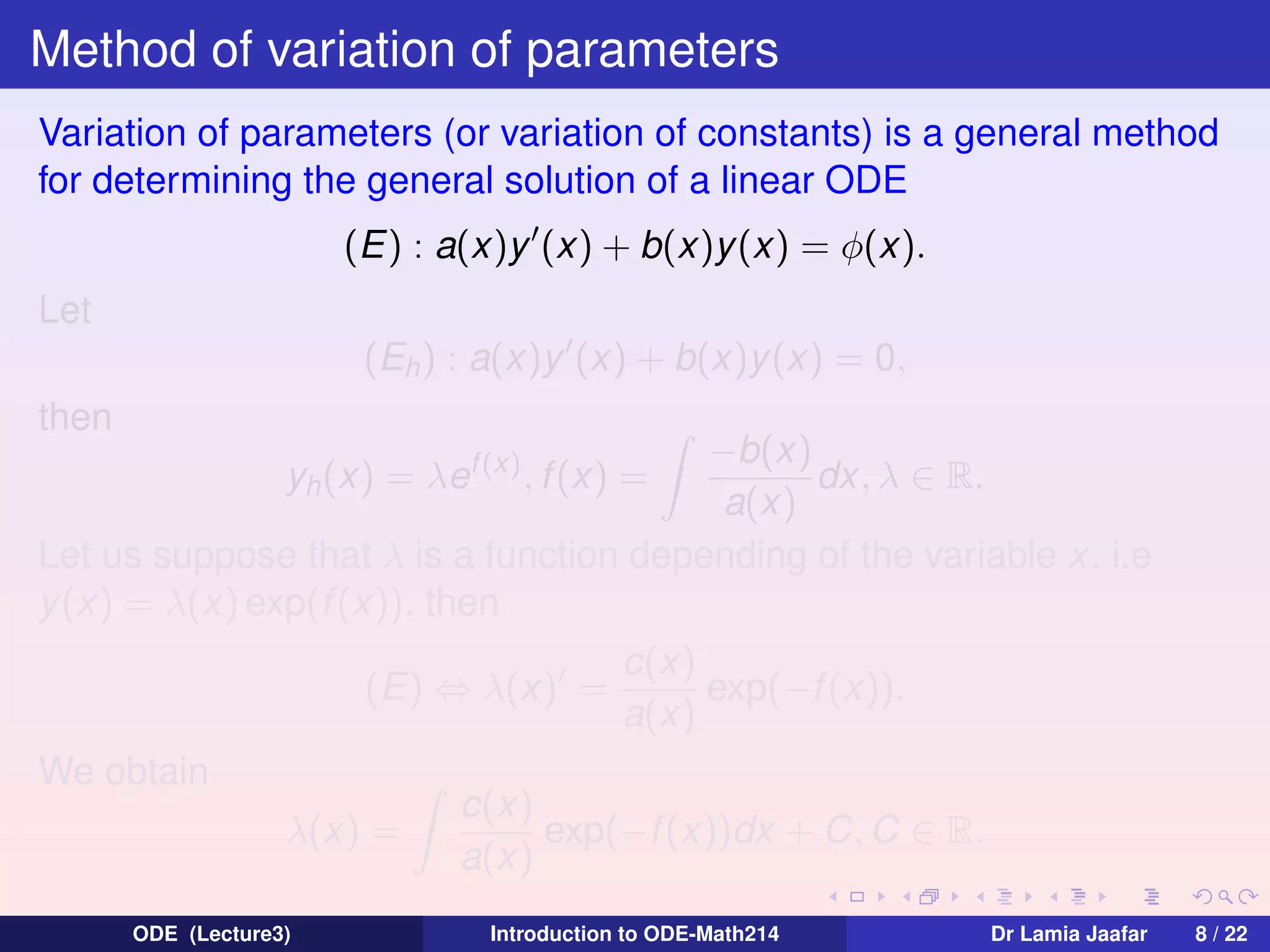
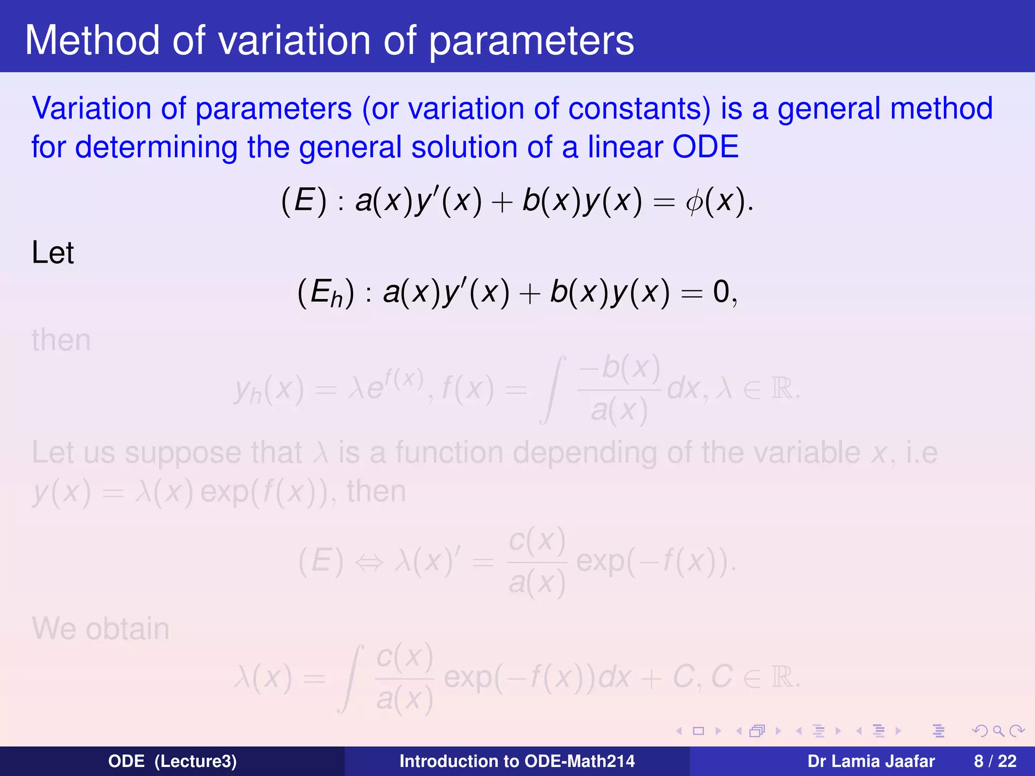
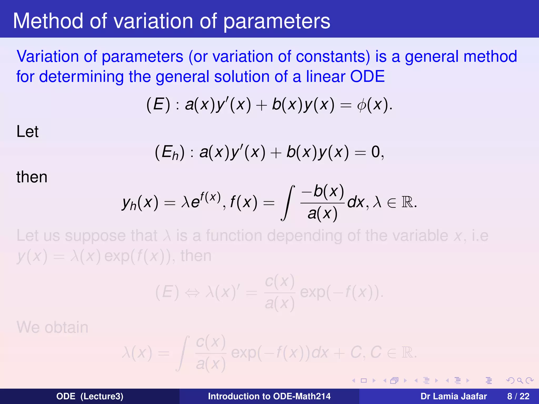
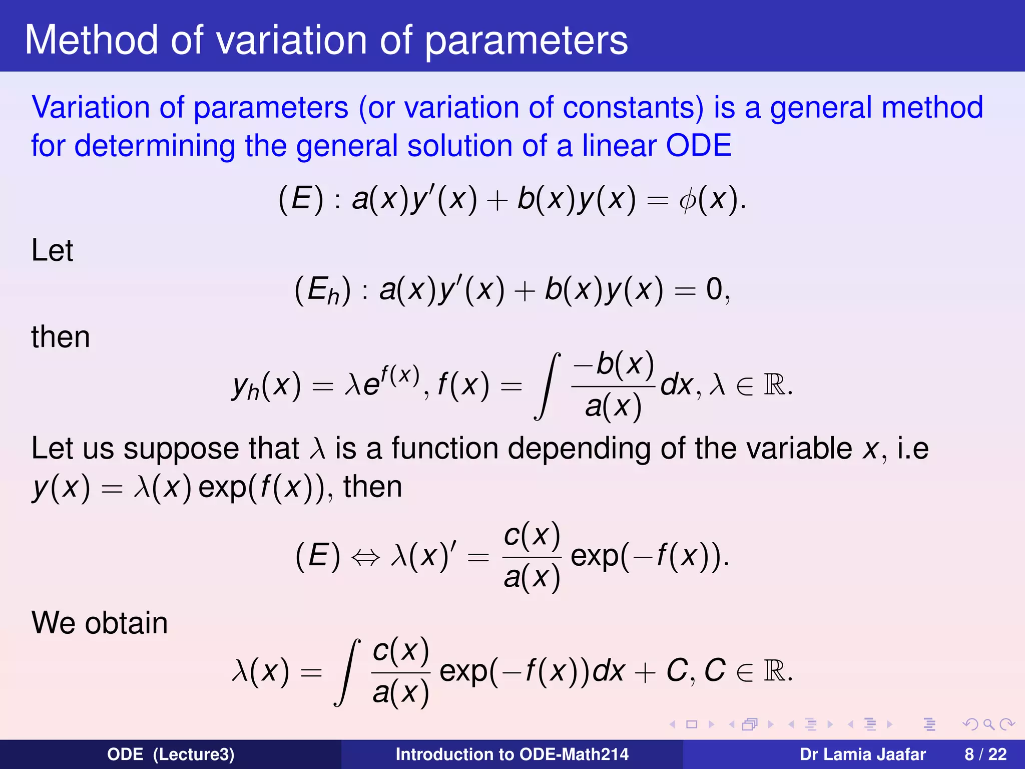
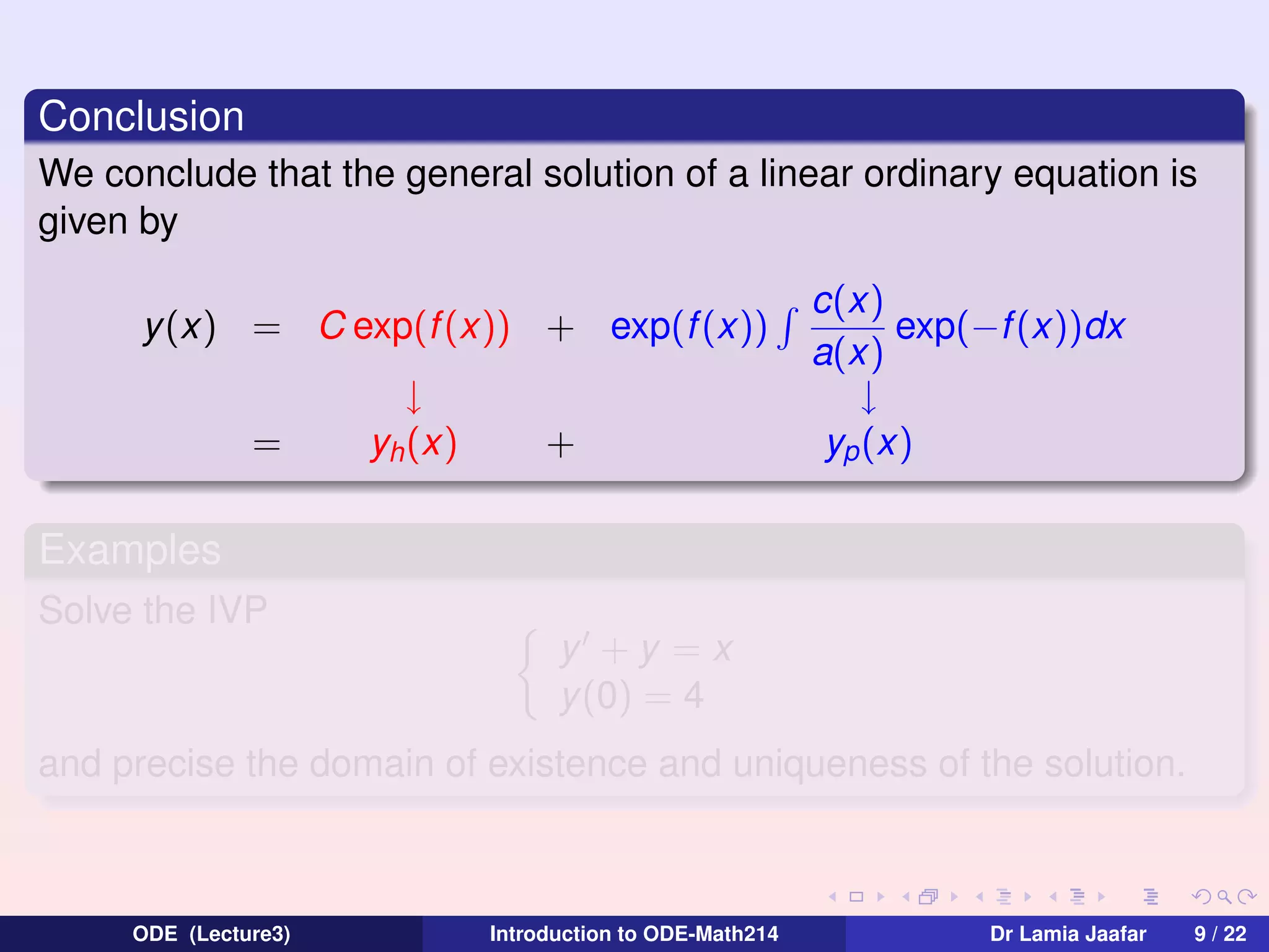
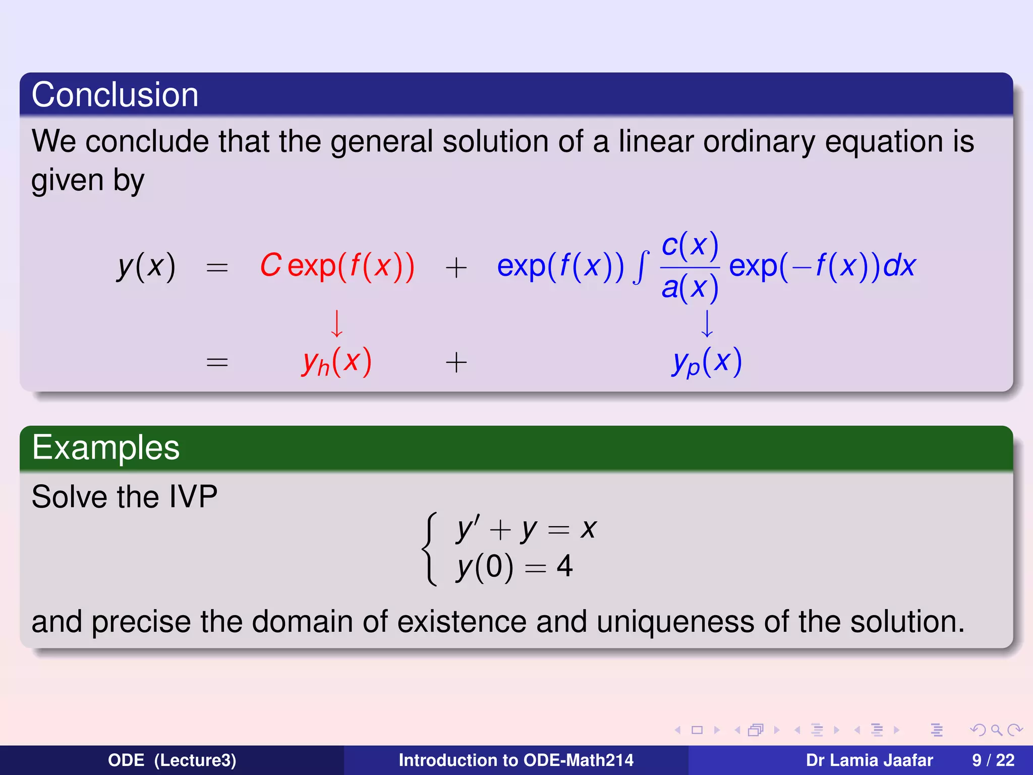
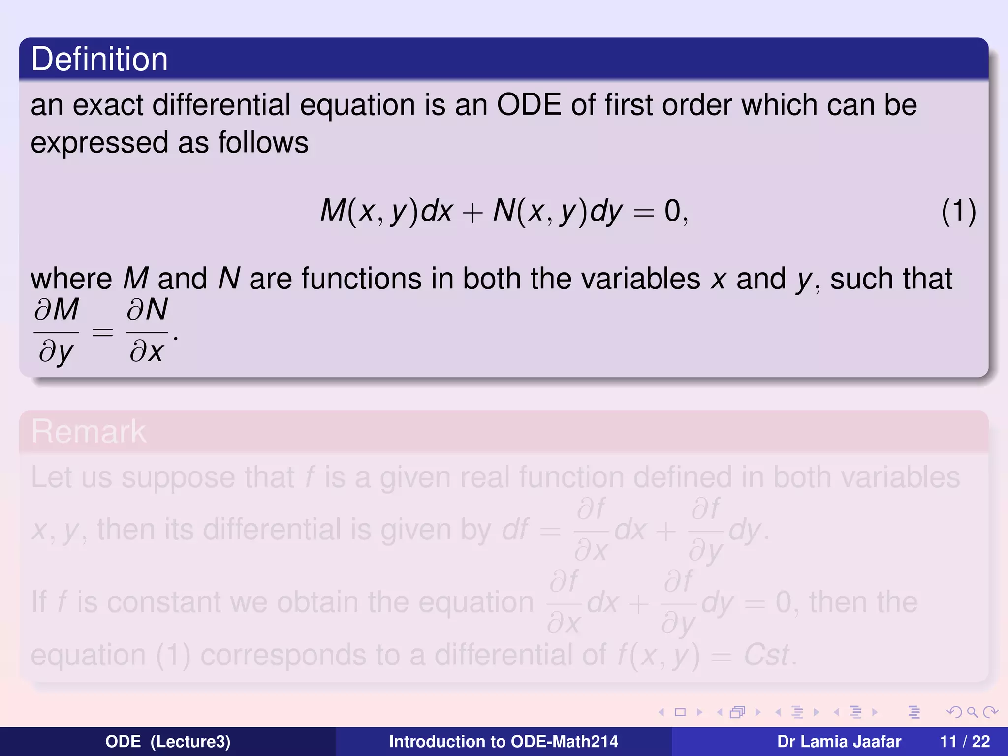
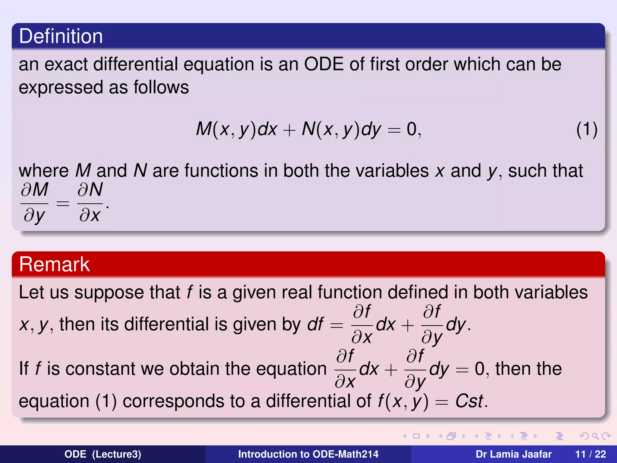
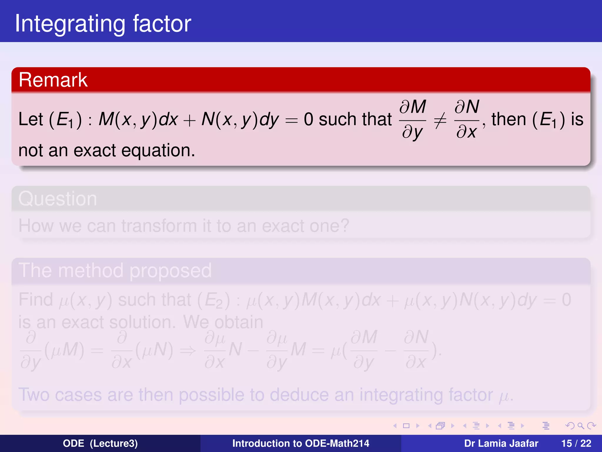
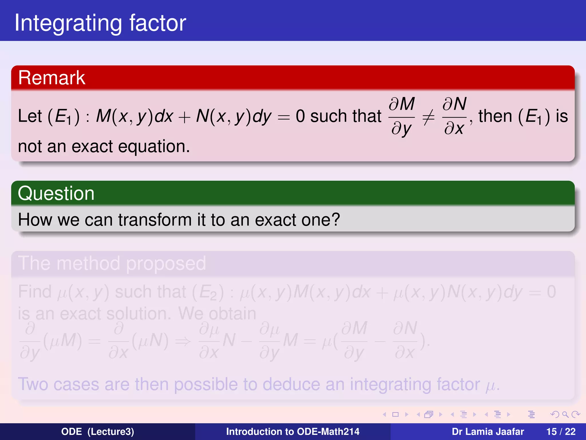
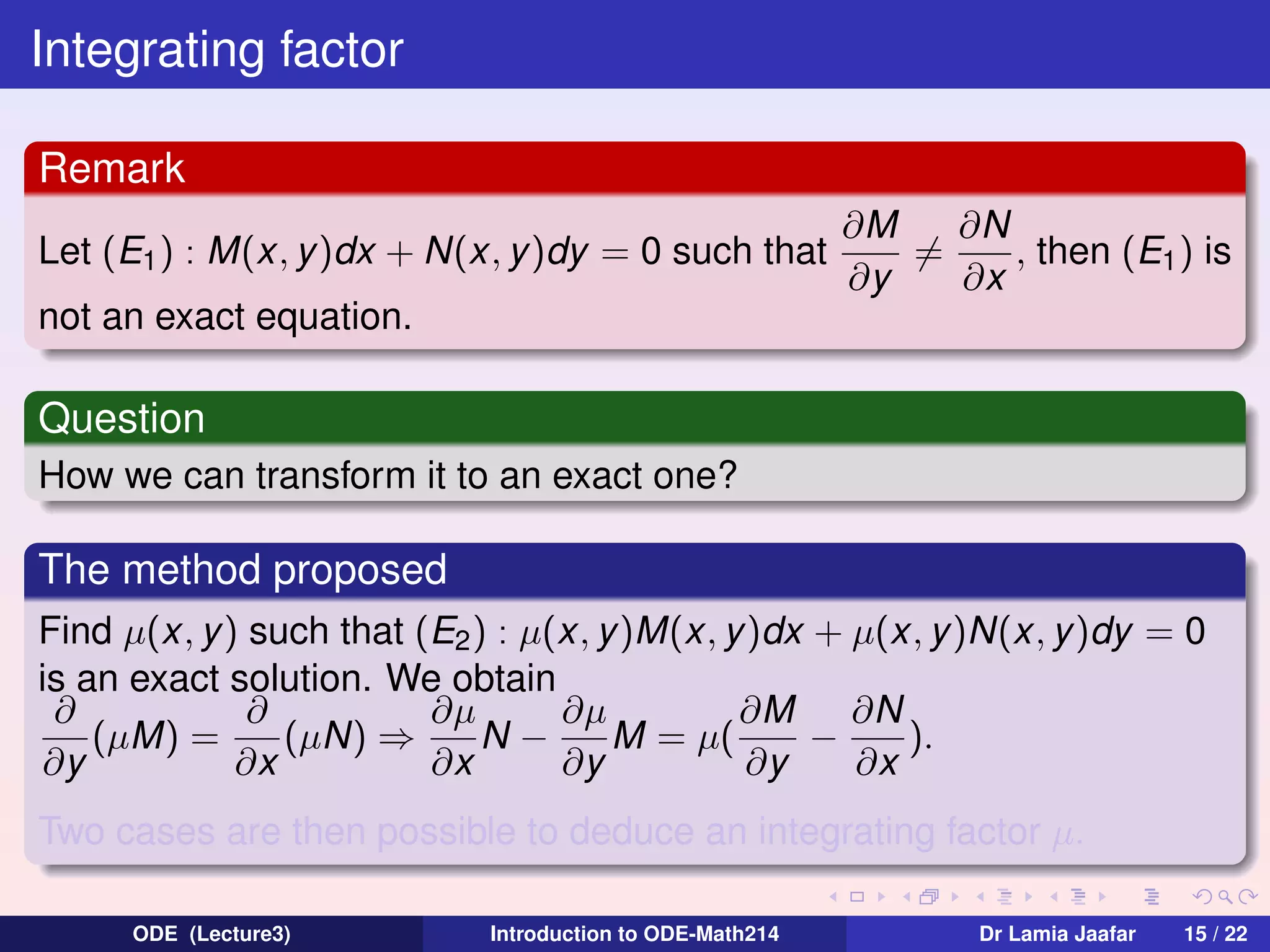
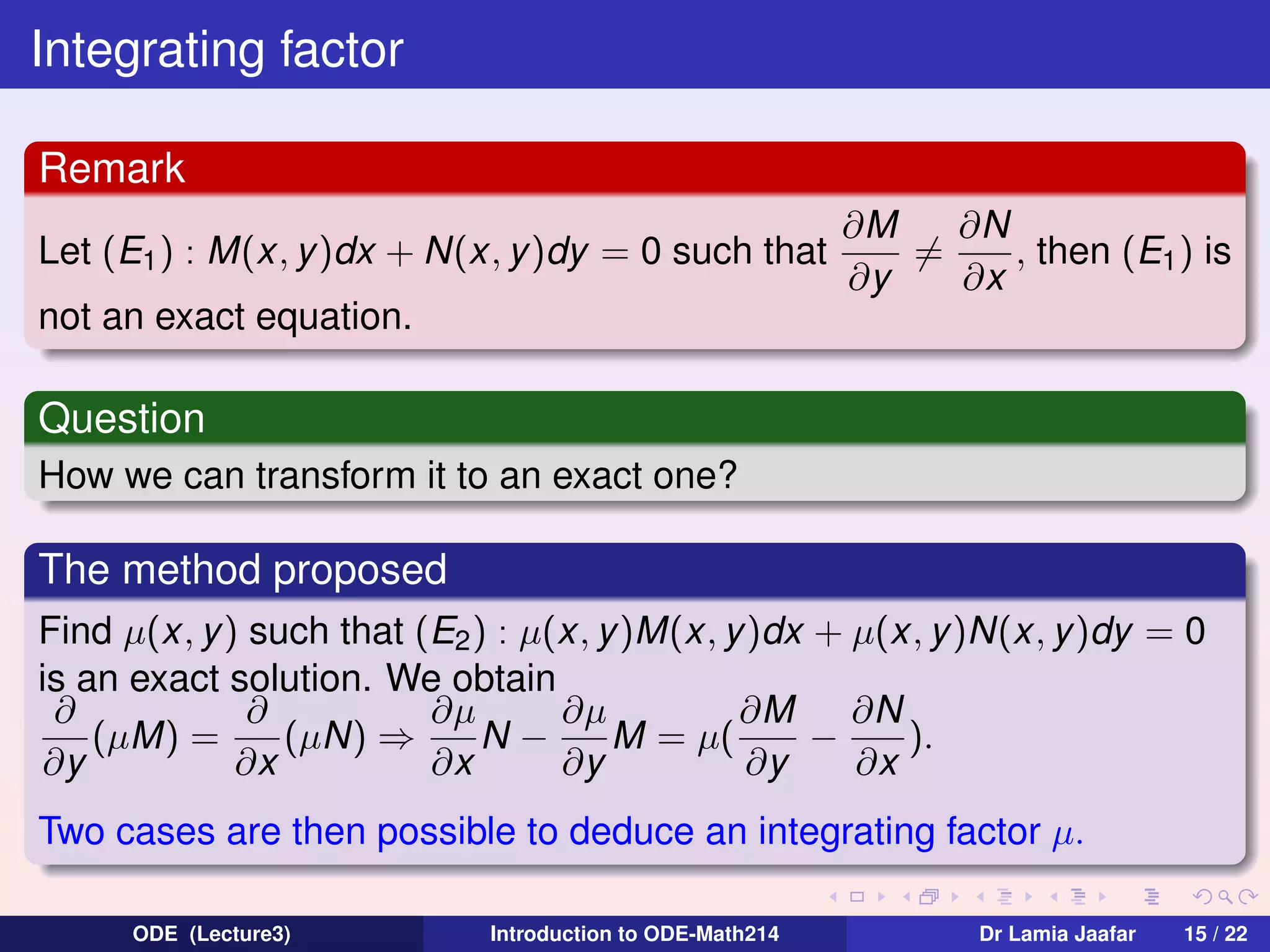
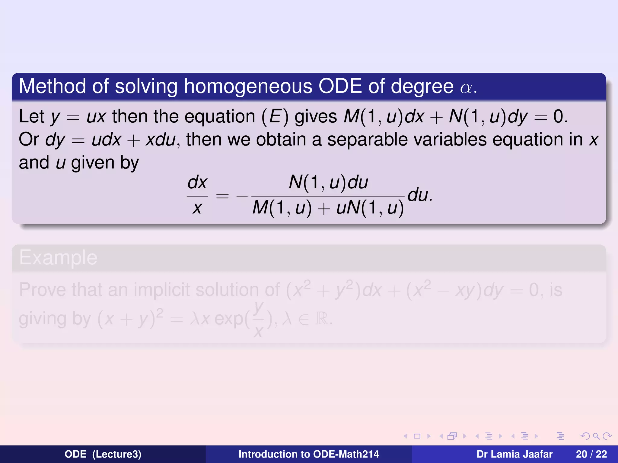
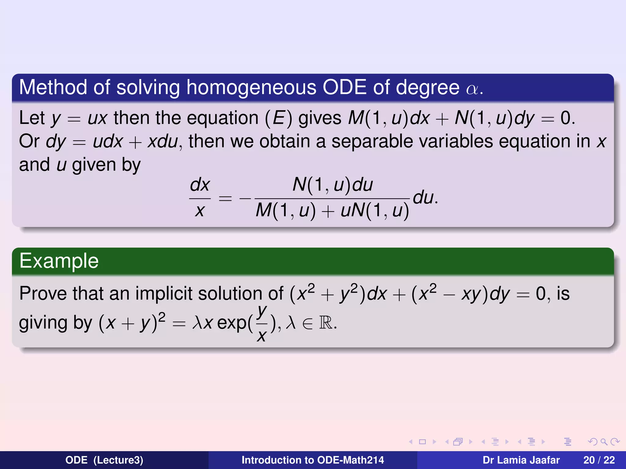
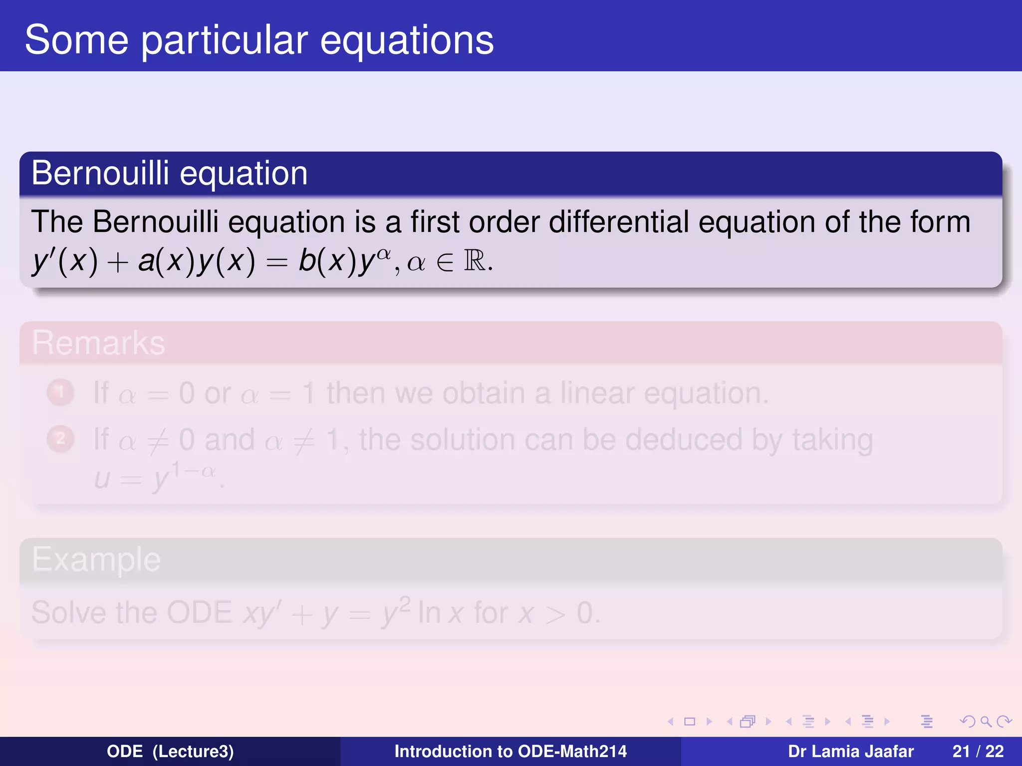
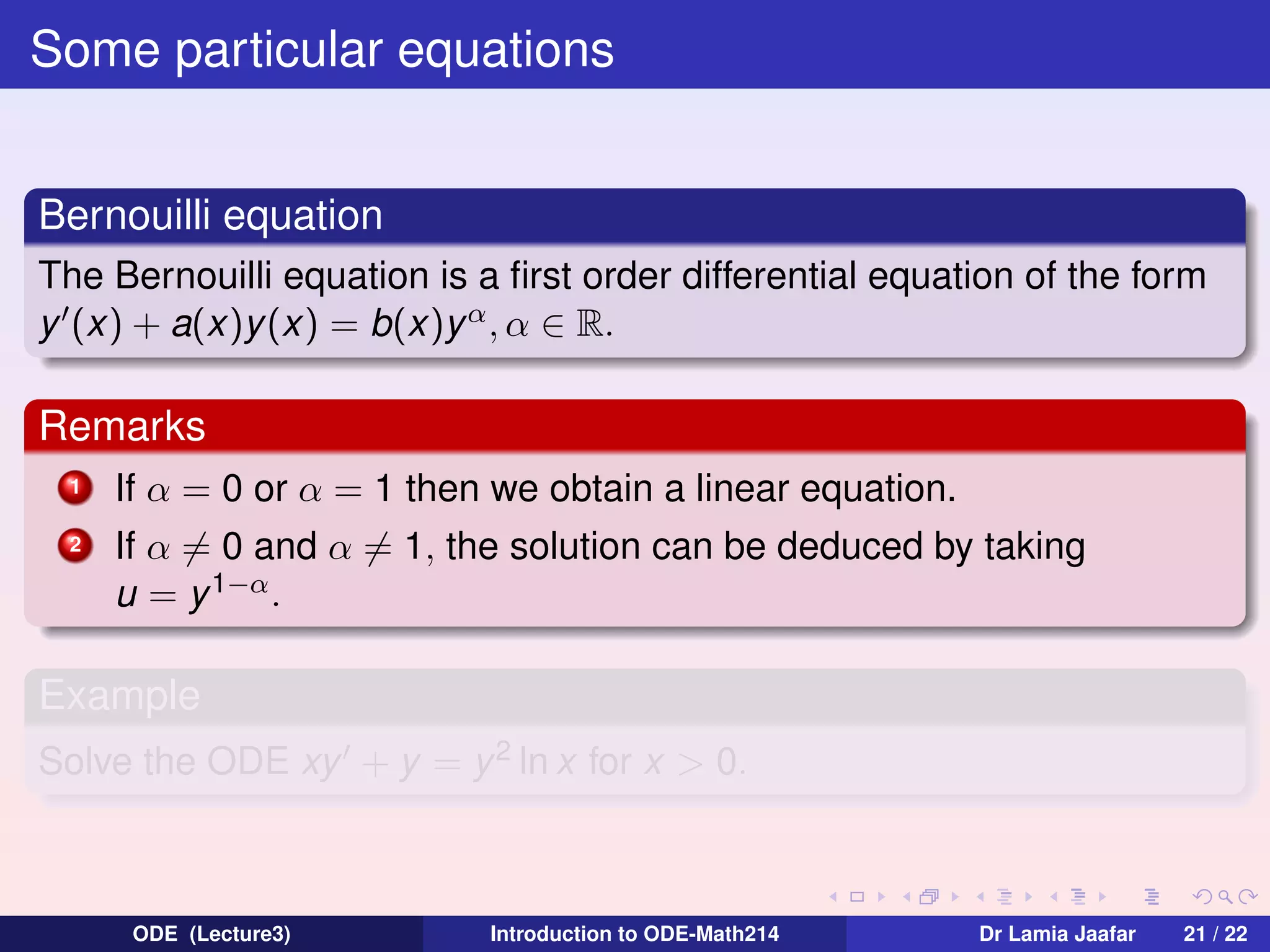
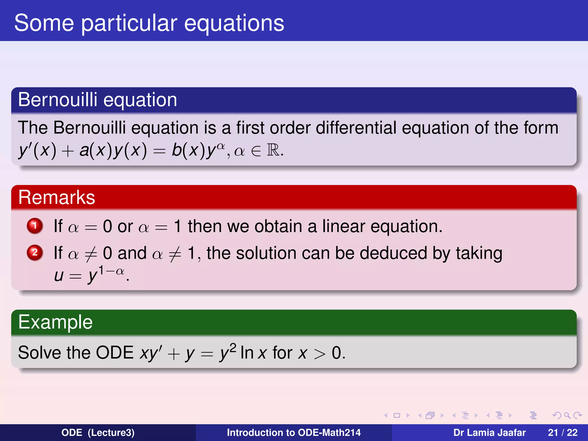
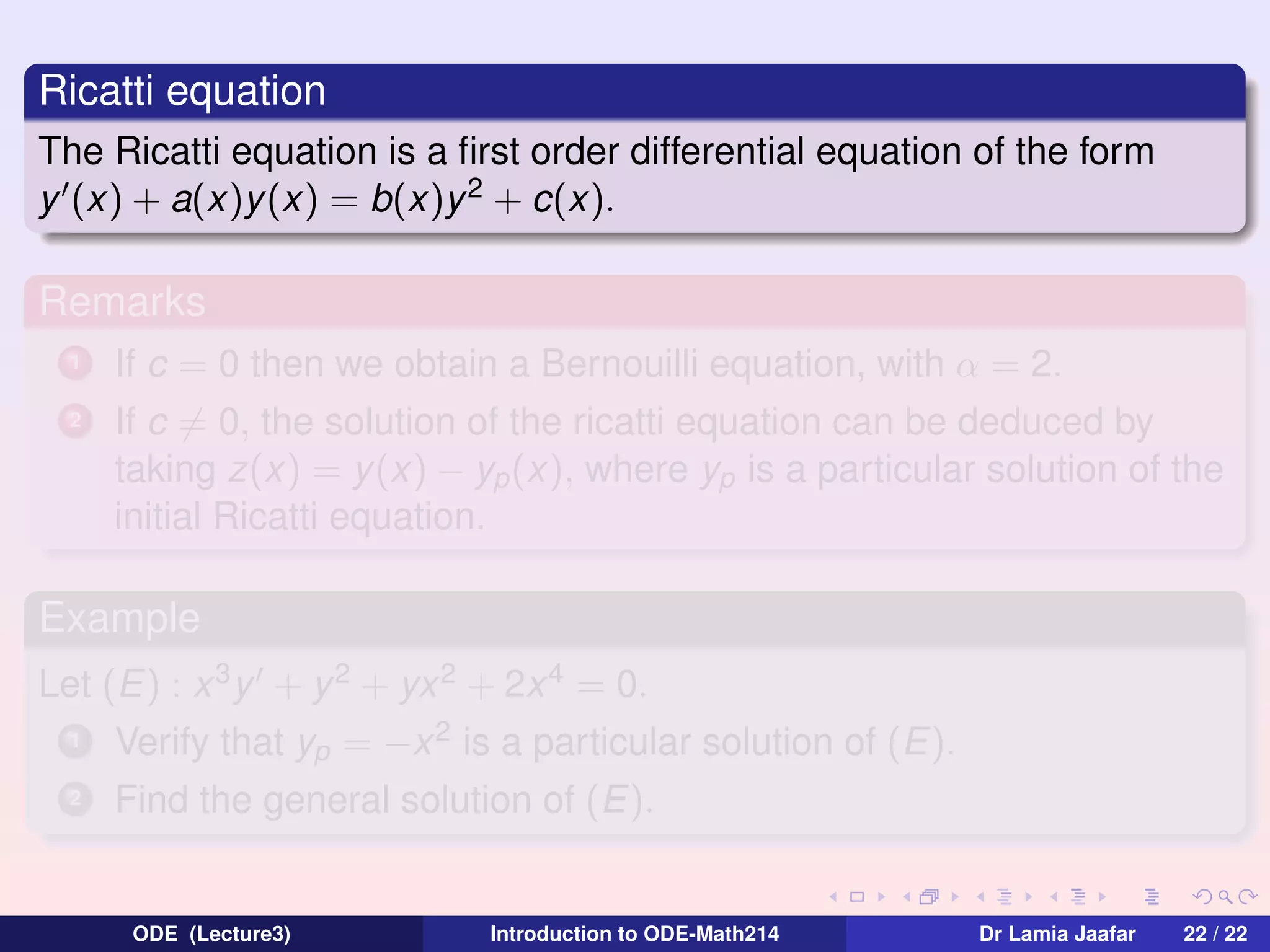
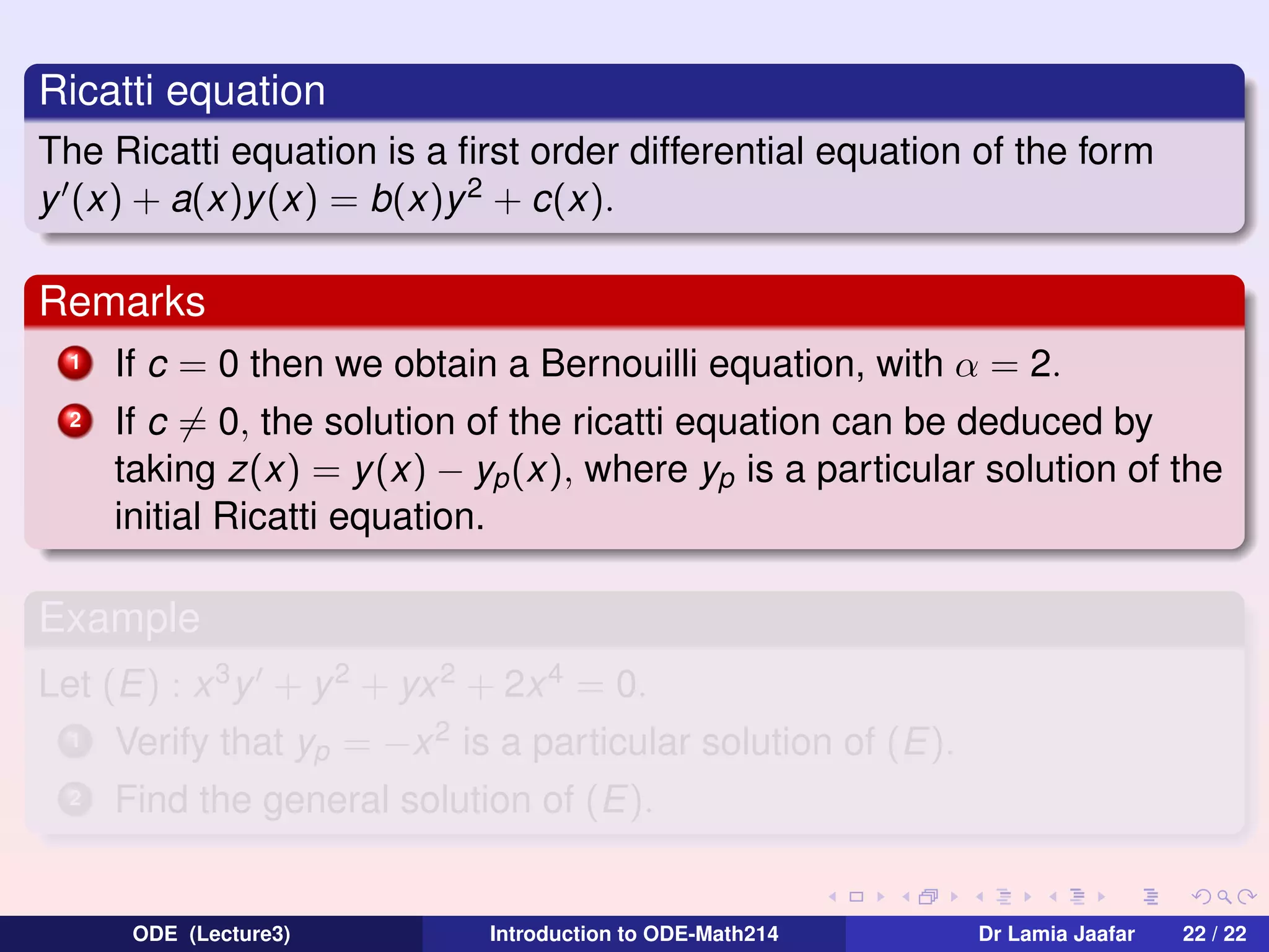
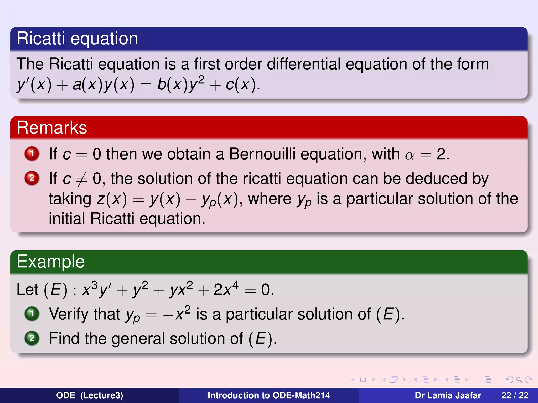
The document provides an overview of first order differential equations and methods for solving them. It discusses linear equations and introduces the method of variation of parameters for finding the general solution to a linear ODE. It also covers exact equations and defines an exact differential equation as one that can be written as M(x,y)dx + N(x,y)dy = 0, where M and N are functions of both x and y and satisfy ∂M/∂y = ∂N/∂x. Examples are provided to demonstrate solving techniques.
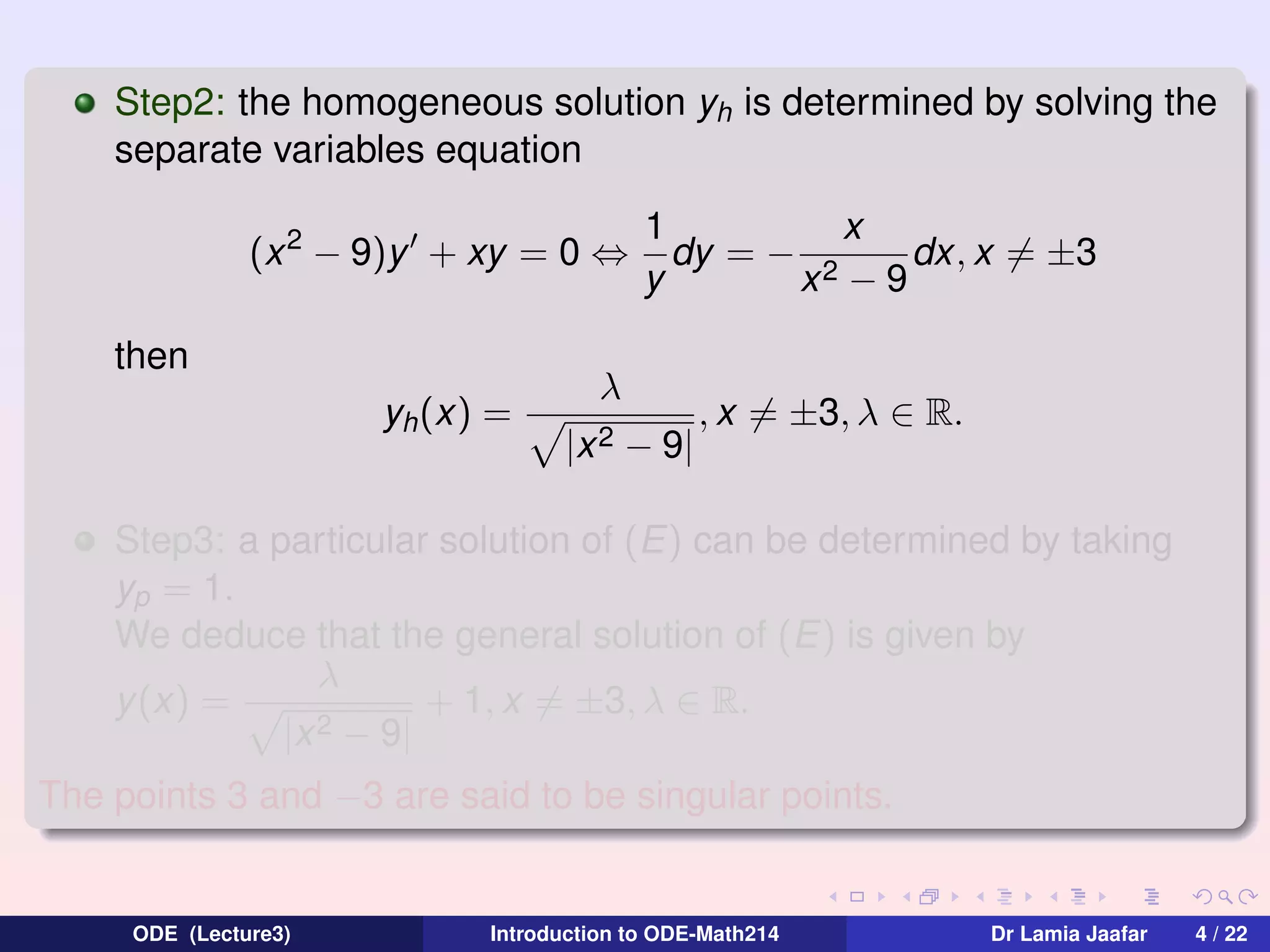
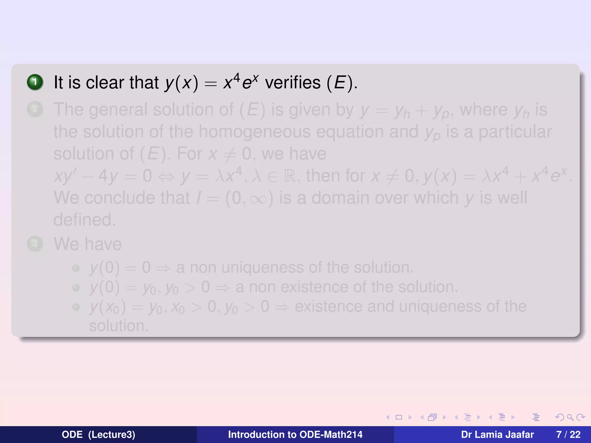
![If x ∈] − ∞, −3[, the general solution is given by
λ
y1 (x) = √
+ 1.
x2 − 9
If x ∈] − 3, 3[, the general solution is given by
λ
+ 1.
y2 (x) = √
9 − x2
If x ∈]3, +∞[, the general solution is given by
λ
+ 1.
y3 (x) = √
2−9
x
1
, we solve the equation on (3, +∞), on which the
4
theorem of existence and uniqueness are assured:
By taking y (5) =
∃!y(x) = √
ODE (Lecture3)
4
x2
−9
+ 1, x ∈ (3, +∞).
Introduction to ODE-Math214
Dr Lamia Jaafar
5 / 22](https://image.slidesharecdn.com/lecture3-ode1lamia-140304162222-phpapp02/75/Lecture3-ode-1-lamia-8-2048.jpg)
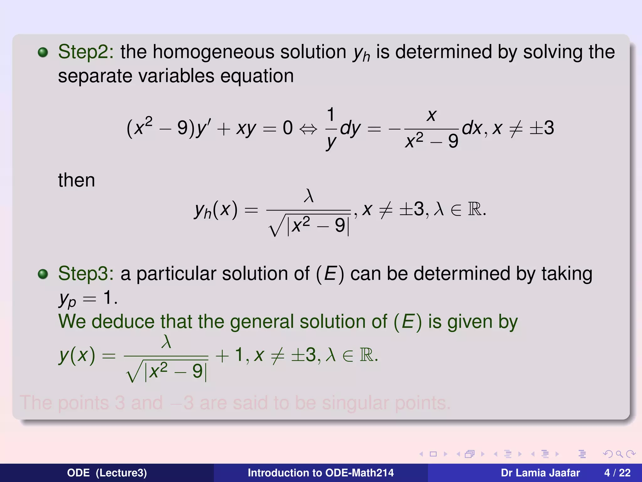
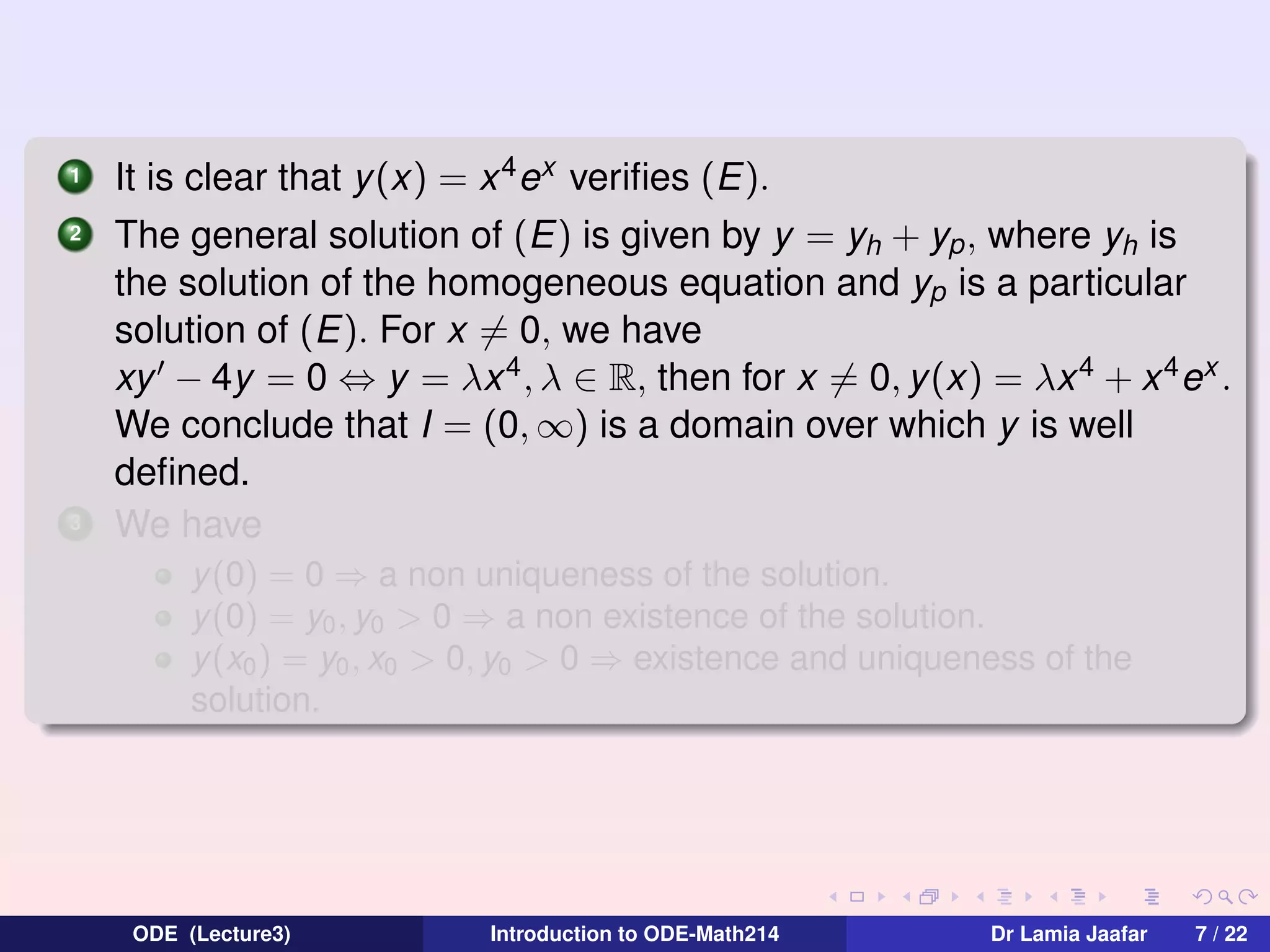
![If x ∈] − ∞, −3[, the general solution is given by
λ
y1 (x) = √
+ 1.
x2 − 9
If x ∈] − 3, 3[, the general solution is given by
λ
+ 1.
y2 (x) = √
9 − x2
If x ∈]3, +∞[, the general solution is given by
λ
+ 1.
y3 (x) = √
2−9
x
1
, we solve the equation on (3, +∞), on which the
4
theorem of existence and uniqueness are assured:
By taking y (5) =
∃!y(x) = √
ODE (Lecture3)
4
x2
−9
+ 1, x ∈ (3, +∞).
Introduction to ODE-Math214
Dr Lamia Jaafar
5 / 22](https://image.slidesharecdn.com/lecture3-ode1lamia-140304162222-phpapp02/75/Lecture3-ode-1-lamia-9-2048.jpg)
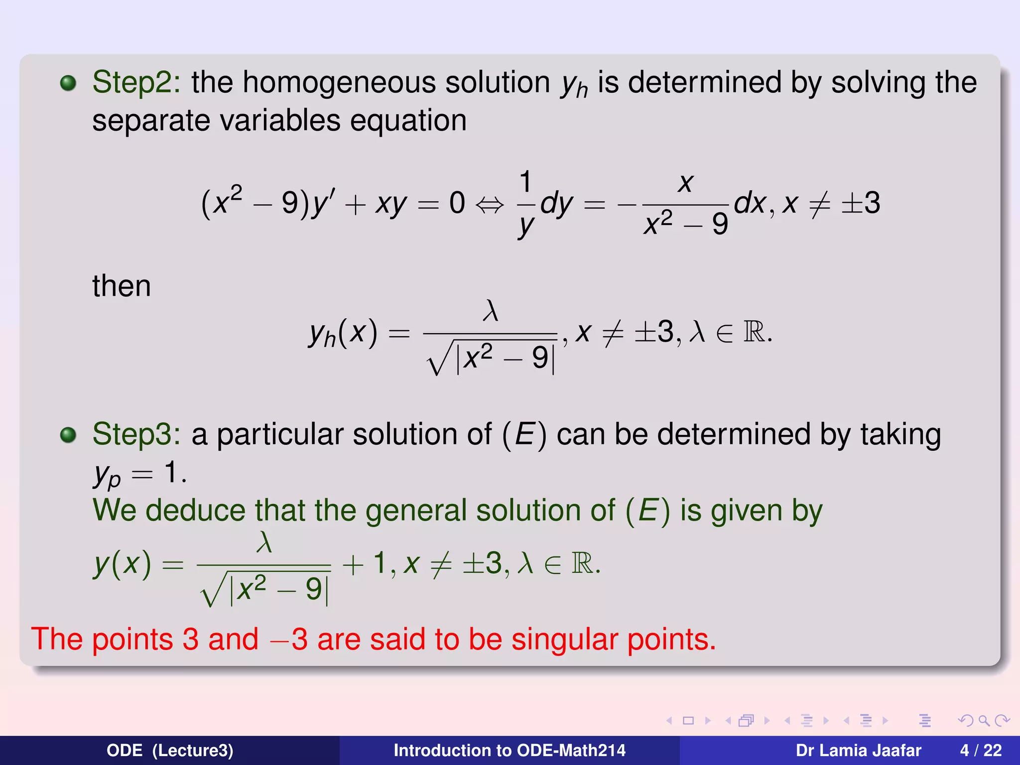
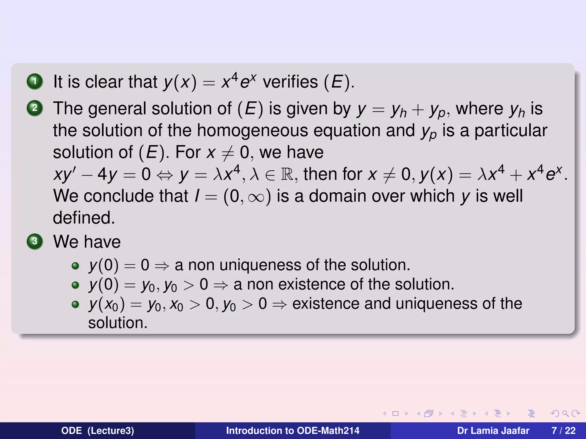
![If x ∈] − ∞, −3[, the general solution is given by
λ
y1 (x) = √
+ 1.
x2 − 9
If x ∈] − 3, 3[, the general solution is given by
λ
+ 1.
y2 (x) = √
9 − x2
If x ∈]3, +∞[, the general solution is given by
λ
+ 1.
y3 (x) = √
2−9
x
1
, we solve the equation on (3, +∞), on which the
4
theorem of existence and uniqueness are assured:
By taking y (5) =
∃!y(x) = √
ODE (Lecture3)
4
x2
−9
+ 1, x ∈ (3, +∞).
Introduction to ODE-Math214
Dr Lamia Jaafar
5 / 22](https://image.slidesharecdn.com/lecture3-ode1lamia-140304162222-phpapp02/75/Lecture3-ode-1-lamia-10-2048.jpg)
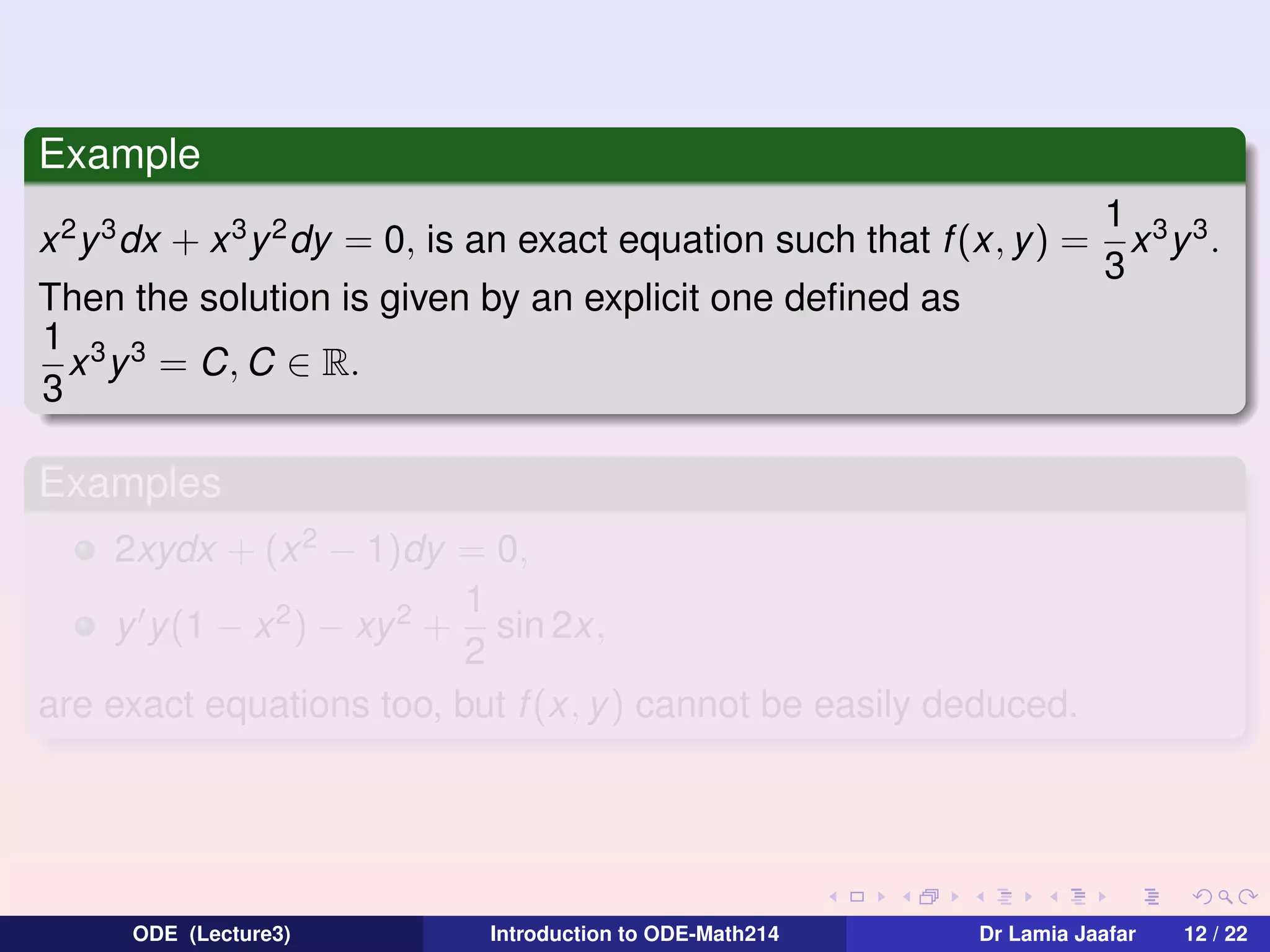
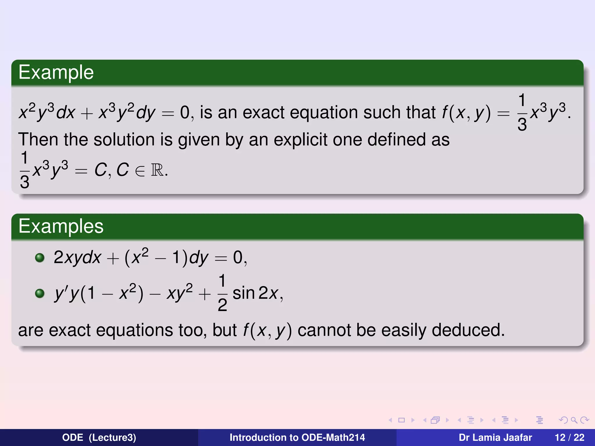
![Solution of (E) : 2xydx + (x 2 − 1)dy = 0
Let M(x, y) = 2xy and N(x, y) = x 2 − 1.
∂M
∂N
As
=
then (E) is an exact equation. We deduce that it exists f
∂y
∂x
defined on a domain I such that
∂f
2
∂x = 2xy,
f (x, y) = x y + F (y),
⇒
∂f
∂f
2−1
= x 2 − 1 = x 2 + F (y )
∂y
∂y = x
we deduce that
F (y) = −1 ⇒ F (y ) = −y + Cst ⇒ f (x, y) = x 2 y − y + Cst, then an
implicit solution is giving by x 2 y − y − C, C ∈ R and an explicit solution
C
is y = 2
, x = ±1.
x −1
The solution of the initial ODE is defined on any interval not containing
either 1 or −1, i.e a domain of the solution y is ] − ∞, −1[ or ] − 1, 1[ or
]1, +∞[.
ODE (Lecture3)
Introduction to ODE-Math214
Dr Lamia Jaafar
14 / 22](https://image.slidesharecdn.com/lecture3-ode1lamia-140304162222-phpapp02/75/Lecture3-ode-1-lamia-28-2048.jpg)
![Solution of (E) : 2xydx + (x 2 − 1)dy = 0
Let M(x, y) = 2xy and N(x, y) = x 2 − 1.
∂M
∂N
As
=
then (E) is an exact equation. We deduce that it exists f
∂y
∂x
defined on a domain I such that
∂f
2
∂x = 2xy,
f (x, y) = x y + F (y),
⇒
∂f
∂f
2−1
= x 2 − 1 = x 2 + F (y )
∂y
∂y = x
we deduce that
F (y) = −1 ⇒ F (y ) = −y + Cst ⇒ f (x, y) = x 2 y − y + Cst, then an
implicit solution is giving by x 2 y − y − C, C ∈ R and an explicit solution
C
is y = 2
, x = ±1.
x −1
The solution of the initial ODE is defined on any interval not containing
either 1 or −1, i.e a domain of the solution y is ] − ∞, −1[ or ] − 1, 1[ or
]1, +∞[.
ODE (Lecture3)
Introduction to ODE-Math214
Dr Lamia Jaafar
14 / 22](https://image.slidesharecdn.com/lecture3-ode1lamia-140304162222-phpapp02/75/Lecture3-ode-1-lamia-29-2048.jpg)


![Week 6 [compatibility mode]](https://cdn.slidesharecdn.com/ss_thumbnails/week6compatibilitymode-130213163919-phpapp02-thumbnail.jpg?width=640&height=640&fit=bounds)


![Week 7 [compatibility mode]](https://cdn.slidesharecdn.com/ss_thumbnails/week7compatibilitymode-130213163717-phpapp02-thumbnail.jpg?width=640&height=640&fit=bounds)


