differentiol equation.pptx

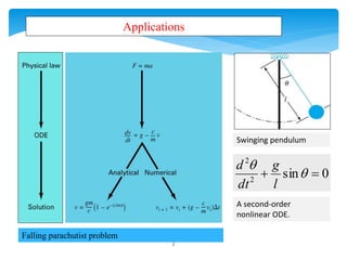
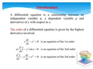
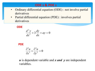
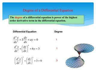
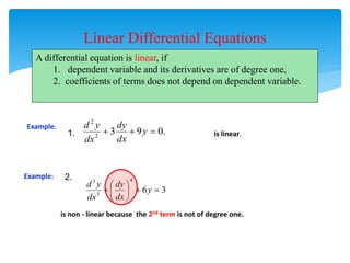
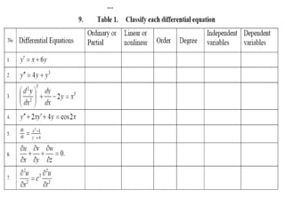
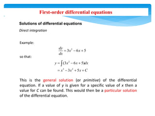
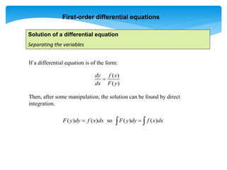
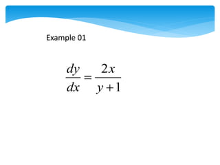
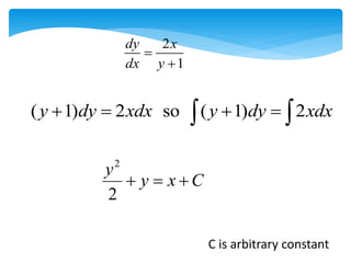
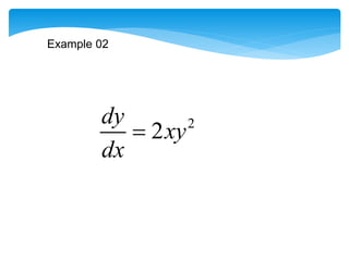
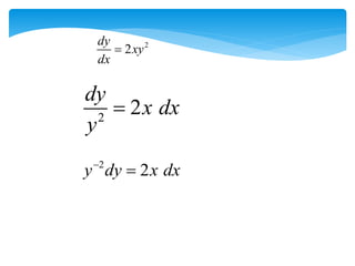
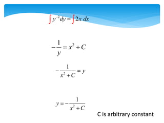
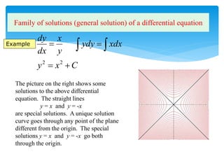
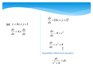
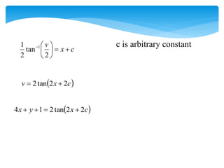
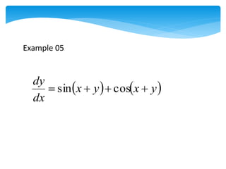
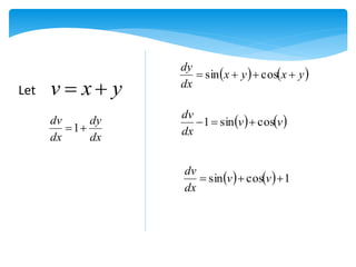
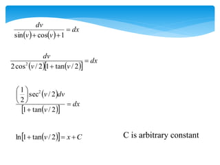
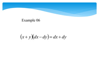
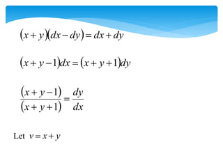
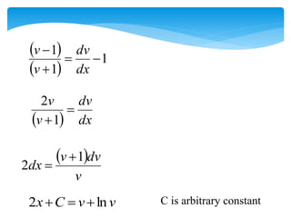
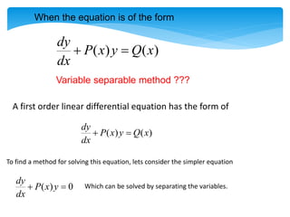
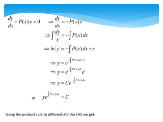
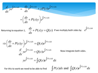
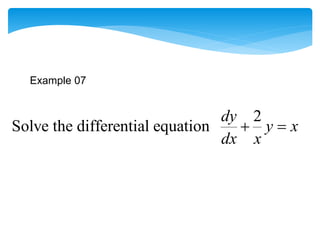
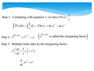
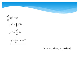
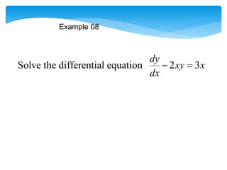
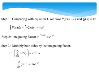
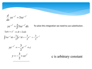
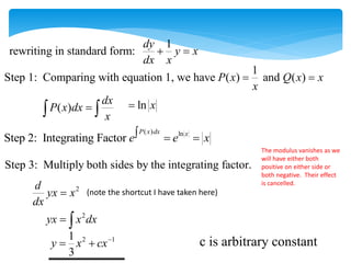
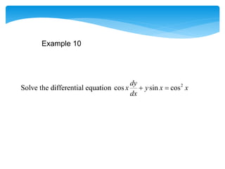
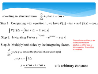
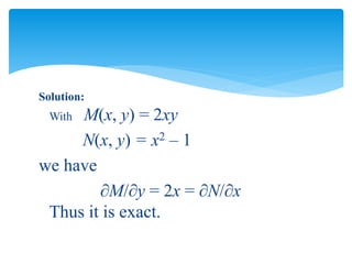
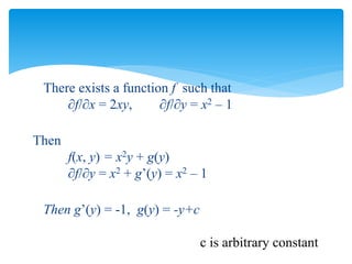
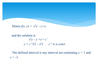
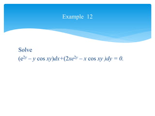
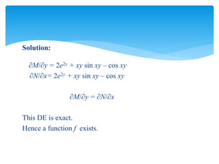
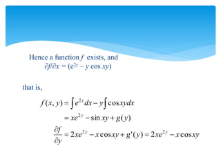
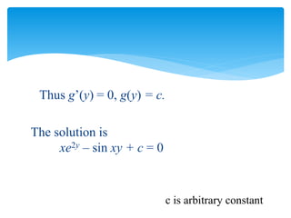
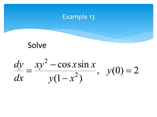
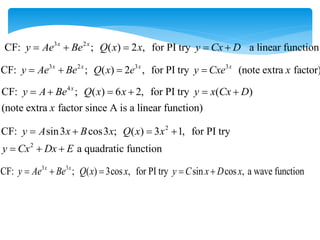
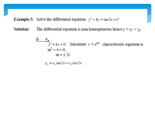
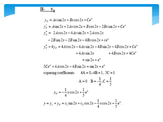
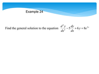
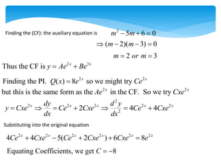
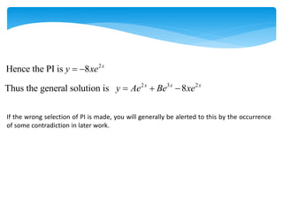
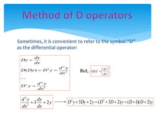
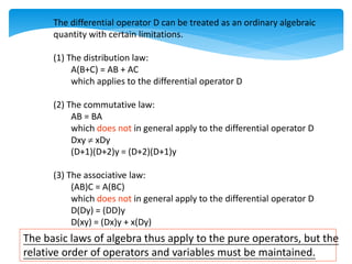
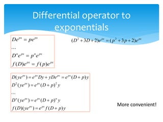
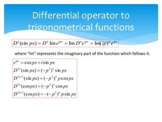
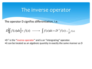
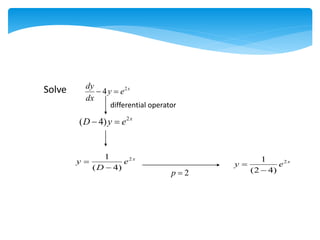
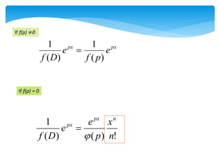
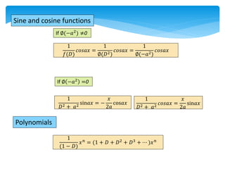
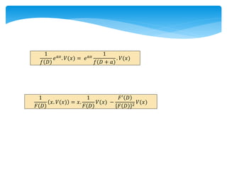
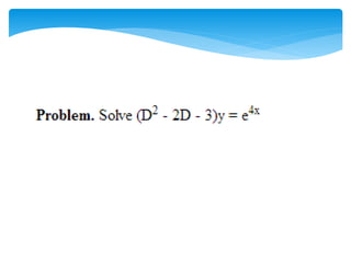
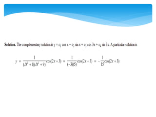
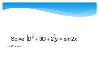
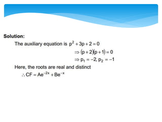
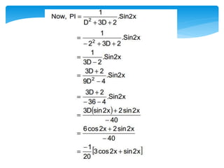
2
Applications
0
sin
2
2

 

l
g
dt
d
Falling parachutist problem
Swinging pendulum
A second-order
nonlinear ODE.

Introduction
A differential equation is a relationship between an
independent variable x, a dependent variable y and
derivatives of y with respect to x.
The order of a differential equation is given by the highest
derivative involved.
2
2
2
2
3
4
3
0 is an equation of the 1st order
sin 0 is an equation of the 2nd order
0 is an equation of the 3rd order
x
dy
x y
dx
d y
xy y x
dx
d y dy
y e
dx dx
 
 
  

0
2
2
2
2






y
u
x
u
• Ordinary differential equation (ODE) : not involve partial
derivatives
• Partial differential equation (PDE) : involves partial
derivatives
ODE
0
3
2
2


 ay
dx
dy
dx
y
d
u is dependent variable and x and y are independent
variables.
PDE
ODE s & PDE s

Degree of a Differential Equation
Differential Equation Degree
0
3
2
2


 ay
dx
dy
dx
y
d
3
6
4
3
3








 y
dx
dy
dx
y
d
0
3
5
3
2
2

















dx
dy
dx
y
d
1
1
3
The degree of a differential equation is power of the highest
order derivative term in the differential equation.

Linear Differential Equations
A differential equation is linear, if
1. dependent variable and its derivatives are of degree one,
2. coefficients of terms does not depend on dependent variable.
Example:
3
6
4
3
3








 y
dx
dy
dx
y
d
is non - linear because the 2nd term is not of degree one.
.
0
9
3
2
2


 y
dx
dy
dx
y
d
Example:
is linear.
1.
2.

First-order differential equations
Solutions of differential equations
Direct integration
Example:
so that:
This is the general solution (or primitive) of the differential
equation. If a value of y is given for a specific value of x then a
value for C can be found. This would then be a particular solution
of the differential equation.
2
3 6 5
dy
x x
dx
  
2
3 2
(3 6 5)
3 5
y x x dx
x x x C
  
   


First-order differential equations
Solution of a differential equation
Separating the variables
If a differential equation is of the form:
Then, after some manipulation, the solution can be found by direct
integration.
( )
( )
dy f x
dx F y

( ) ( ) so ( ) ( )
F y dy f x dx F y dy f x dx
 
 

2
1
dy x
dx y


Example 01

2
1
dy x
dx y


( 1) 2 so ( 1) 2
y dy xdx y dy xdx
   
 
C is arbitrary constant
C
x
y
y



2
2

2
2
dy
xy
dx

2
2
dy
x dx
y

2
2
y dy x dx



2
2
y dy x dx


 
2
1
x C
y
  
2
1
y
x C
 

2
1
y
x C
 


C
x
y
xdx
ydy
y
x
dx
dy



  
2
2
Family of solutions (general solution) of a differential equation
Example
The picture on the right shows some
solutions to the above differential
equation. The straight lines
y = x and y = -x
are special solutions. A unique solution
curve goes through any point of the plane
different from the origin. The special
solutions y = x and y = -x go both
through the origin.

Example 03
 
2
2
2 1 x
dy
x y e
dx
 

 
2
2
2 1 x
dy
x y e
dx
 
2
2
1
2
1
x
dy x e dx
y


Separable differential equation
2
2
1
2
1
x
dy x e dx
y


 
2
1
tan x
y e C

 

Example (cont.):
 
2
2
2 1 x
dy
x y e
dx
 
2
1
tan x
y e C

  Now we have y as an implicit function of x.
We can find y as an explicit function of x by
taking the tangent of both sides.
   
2
1
tan tan tan x
y e C

 
 
2
tan x
y e C
 

 2
1
4 

 y
x
dx
dy
Example 04

Separable differential equation
1
4 

 y
x
v
 2
1
4 

 y
x
dx
dy
dx
dy
dx
dv

 4 2
4 v
dx
dv


4
2

 v
dx
dv
let
dx
v
dv

 4
2

c
x
v









2
tan
2
1 1
 
c
x
v 2
2
tan
2 

 
c
x
y
x 2
2
tan
2
1
4 



c is arbitrary constant

   
y
x
y
x
dx
dy



 cos
sin
Example 05

   
y
x
y
x
dx
dy



 cos
sin
y
x
v 

dx
dy
dx
dv

1
   
v
v
dx
dv
cos
sin
1 


    1
cos
sin 

 v
v
dx
dv
Let

   
dx
v
v
dv


 1
cos
sin
   
 
dx
v
v
dv

 2
/
tan
1
2
/
cos
2 2
 
 
 
dx
v
dv
v








2
/
tan
1
2
/
sec
2
1 2
 
  C
x
v 

 2
/
tan
1
ln C is arbitrary constant

   dy
dx
dy
dx
y
x 



Example 06

   dy
dx
dy
dx
y
x 



   dy
y
x
dx
y
x 1
1 




 
  dx
dy
y
x
y
x





1
1
y
x
v 

Let

 
 
1
1
1




dx
dv
v
v
  dx
dv
v
v

1
2
 
v
dv
v
dx
1
2


v
v
C
x ln
2 

 C is arbitrary constant

A first order linear differential equation has the form of
( ) ( )
dy
P x y Q x
dx
 
To find a method for solving this equation, lets consider the simpler equation
( ) 0
dy
P x y
dx
  Which can be solved by separating the variables.
( ) ( )
dy
P x y Q x
dx
 
When the equation is of the form
Variable separable method ???

( ) 0
dy
P x y
dx
  ( )
dy
P x y
dx
  
( )
dy
P x dx
y
  
 
ln ( )
y P x dx c
   

( )
P x dx c
y e
 

 
( )
P x dx c
y e e

 
( )
P x dx
y Ce

 
or
( )
P x dx
ye C
 
Using the product rule to differentiate the LHS we get:

( )
P x dx
d
ye
dx
 
( ) ( )
( )
P x dx P x dx
dy
e yP x e
dx
 

( )
( )
P x dx
dy
P x y e
dx
  
 
 
 
Returning to equation 1, ( ) ( )
dy
P x y Q x
dx
  If we multiply both sides by
( )
P x dx
e
( ) ( )
( ) ( )
P x dx P x dx
dy
P x y e Q x e
dx
   
  
 
 
( ) ( )
( )
P x dx P x dx
d
ye Q x e
dx
 
 Now integrate both sides.
( ) ( )
( )
P x dx P x dx
ye Q x e dx
 
 
For this to work we need to be able to find
( )
( ) and ( )
P x dx
P x dx Q x e dx

 

2
Solve the differential equation
dy
y x
dx x
 
Example 07

2
Step 1: Comparing with equation 1, we have ( )
P x
x

2
( )
P x dx dx
x

  2ln x

2
ln x
 2
ln x

2
( ) ln
Step 2:
P x dx x
e e
  2
x
  
( )
is called the integrating factor
P x dx
e
Step 3: Multiply both sides by the integrating factor.
2 2
2
dy
x y x x
dx x
 
 
 
 
2 3
d
yx x
dx


2 3
d
yx x
dx

2 3
yx x dx
 
4
2
4
x
yx c
 
2 2
1
4
y x cx
 

Example 08
Solve the differential equation 2 3
dy
xy x
dx
 

Step 1: Comparing with equation 1, we have ( ) 2 and ( ) 3
P x x Q x x
  
( ) 2
P x dx xdx
 
 
2
x
 
2
( )
Step 2: Integrating Factor
P x dx x
e e
 
2 2
2 3
x x
dy
e xy e x
dx
 
 
 
 
 
2 2
3
x x
d
ye xe
dx
 


2 2
3
x x
d
ye xe
dx
 

2 2
3
x x
ye xe dx
 
  To solve this integration we need to use substitution.
2
Let t x
 2
dt xdx
 
2 3
3
2
x t
xe dx e dt
 

 
3
2
t
e
 
2
3
2
x
e
 
2 2
3
2
x x
ye e c
 
  
2
3
2
x
y ce
   c is arbitrary constant

Example 09
2 3
Solve the differential equation 0
dy
x x xy
dx
  

1
Step 1: Comparing with equation 1, we have ( ) and ( )
P x Q x x
x
 
( )
dx
P x dx
x

  ln x

( ) ln
Step 2: Integrating Factor
P x dx x
e e x
  
2
d
yx x
dx

1
rewriting in standard form:
dy
y x
dx x
 
(note the shortcut I have taken here)
2
yx x dx
 
2 1
1
3
y x cx
 
The modulus vanishes as we
will have either both
positive on either side or
both negative. Their effect
is cancelled.

Example 10
2
Solve the differential equation cos sin cos
dy
x y x x
dx
 

Step 1: Comparing with equation 1, we have ( ) tan and ( ) cos
P x x Q x x
 
( ) tan
P x dx xdx

  ln sec x

( ) lnsec
Step 2: Integrating Factor sec
P x dx x
e e x
  
sec 1
d
y x
dx

rewriting in standard form: tan cos
dy
y x x
dx
 
(note the shortcut I have taken here)
sec 1
y x dx
 
cos cos
y x x c x
 
The modulus vanishes as we
will have either both
positive on either side or
both negative. Their effect
is cancelled.

Differential of a Function of n Variables
 If z = f(x, y), its differential or total differential is
 Now if z = f(x, y) = c,
dy
y
f
dx
x
f
dz






0


















dy
y
f
dx
x
f
n
n
dx
x
f
dx
x
f
dx
x
f
dx
x
f
dz












 ...
3
3
2
2
1
1

Definition
M(x, y) dx + N(x, y) dy is an exact differential
in a region R of the xy-plane, if it corresponds to the
differential of some function f(x, y). A first-order DE
of the form
M(x, y) dx + N(x, y) dy = 0
is said to be an exact equation, if the left side is an
exact differential.
Exact Equation

Let M(x, y) and N(x, y) be continuous and have
continuous first partial derivatives in a region R defined
by a < x < b, c < y < d. Then a necessary and
sufficient condition that M(x, y) dx + N(x, y) dy be an
exact differential is
Criterion for an Exact Differential
x
N
y
M






Example 11
Solve
2xy dx + (x2 – 1) dy = 0.

Solution:
With M(x, y) = 2xy
N(x, y) = x2 – 1
we have
M/y = 2x = N/x
Thus it is exact.

There exists a function f such that
f/x = 2xy, f/y = x2 – 1
Then
f(x, y) = x2y + g(y)
f/y = x2 + g’(y) = x2 – 1
Then g’(y) = -1, g(y) = -y+c

Hence f(x, y) = x2y – y+c,
and the solution is
x2y – y +c= c’
y = c”/(1 – x2) c” is a const
The defined interval is any interval not containing x = 1 and
x = -1.

Example 12
Solve
(e2y – y cos xy)dx+(2xe2y – x cos xy )dy = 0.

Solution:
M/y = 2e2y + xy sin xy – cos xy
N/x= 2e2y + xy sin xy – cos xy
M/y = N/x
This DE is exact.
Hence a function f exists.

Hence a function f exists, and
f/x = (e2y – y cos xy)
that is,
xy
x
xe
y
g
xy
x
xe
y
f
y
g
xy
xe
xydx
y
dx
e
y
x
f
y
y
y
y
cos
2
)
(
'
cos
2
)
(
sin
cos
)
,
(
2
2
2
2











 


Thus g’(y) = 0, g(y) = c.
The solution is
xe2y – sin xy + c = 0

Example 13
2
)
0
(
,
)
1
(
sin
cos
2
2



 y
x
y
x
x
xy
dx
dy
Solve

Solution:
Rewrite the DE in the form
(cos x sin x – xy2) dx + y(1 – x2) dy = 0
Since
M/y = – 2xy = N/x
(This DE is exact)

Now f/x=cosxsinx-xy2
f(x, y)=-(cos2x)/2- x2y2/2+g(y)
f/y = -xy2+g’(y)=y(1 – x2)
g’(y)=y then g(y)= y2/2

We have
f(x, y)=-(cos2x)/2- x2y2/2+y2/2
or
y2(1 – x2) – cos2 x = c’
where c’= 2(c1 -c). Now y(0) = 2, so c’= 3.
The solution is
y2(1 – x2) – cos2 x = 3

 It is sometimes possible to find an integrating factor
(x, y), such that
(x, y)M(x, y)dx + (x, y)N(x, y)dy = 0
is an exact differential.
Equation above is exact if and only if
(M)y = (N)x
Then
My + yM = Nx + xN,
or
xN – yM = (My – Nx) 
Integrating Factors

Initial conditions
 In many physical problems we need to find the particular
solution that satisfies a condition of the form y(x0)=y0.
This is called an initial condition, and the problem of
finding a solution of a differential equation that satisfies
the initial condition is called an initial-value problem.
Example : Find a solution to ydy/dx = x satisfying the
initial condition y(0) = 2.

 Example (cont.): Find a solution to ydy/dx = x satisfying
the initial condition y(0) = 2.
y2/2=x2 /2+ C
22 /2= 02 /2+ C
C = 2
y2 = x2 + 4

A population of living creatures normally increases at a
rate that is proportional to the current level of the
population. Other things that increase or decrease at a
rate proportional to the amount present include
radioactive material and money in an interest-bearing
account.
If the rate of change is proportional to the amount
present, the change can be modeled by:
dy
ky
dt

Law of natural growth or decay

dy
ky
dt

1
dy k dt
y

1
dy k dt
y

 
ln y kt C
 
Rate of change is proportional to the
amount present.
Divide both sides by y.
Integrate both sides.
ln y kt C
e e 
 Exponentiate both sides.
C kt
y e e
 
C kt
y e e
 
kt
y Ae


Real-life populations do not increase forever. There is some limiting factor
such as food or living space.
There is a maximum population, or carrying capacity, M.
A more realistic model is the logistic growth model where growth rate is
proportional to both the size of the population (y) and the amount by which y
falls short of the maximal size (M-y). Then we have the equation:
)
( y
M
ky
dt
dy


Logistic Growth Model
The solution to this differential equation is given by
)
0
(
where
,
)
(
0
0
0
0
y
y
e
y
M
y
M
y
y kMt



 

When ( ) 0 then the equations are non-homogeneous.
Q x 
2
2
Differential equations of the form ( )
are called second order linear differential equations.
d y dy
a b cy Q x
dx dx
  
When ( ) 0 then the equations are referred to as homogeneous,
Q x 

Theorem
If ( ) and ( ) are two solutions then so is ( ) ( )
y f x y g x y f x g x
   
Proof
2 2
2 2
0
d f df d g dg
a b cf a b cg
dx dx dx dx
     
2
2
and 0
d g dg
a b cg
dx dx
  
Adding:
2
2
we have 0
d f df
a b cf
dx dx
  
 
2 2
2 2
0
d f d g df dg
a b c f g
dx dx dx dx
   
     
 
 
 
 
And so ( ) ( ) is a solution to the differential equation.
y f x g x
 

, for and , is a solution to the equation 0
mx dy
y Ae A m b cy
dx
  
It is reasonable to consider it as a possible solution for
2
2
0
d y dy
a b cy
dx dx
  
mx
y Ae
 mx
dy
Ame
dx
 
2
2
2
mx
d y
Am e
dx
 
If is a solution it must satisfy
mx
y Ae
 2
0
mx mx mx
aAm e bAme cAe
  
assuming 0, then by division we get
mx
Ae 
2
0
am bm c
   Auxiliary equation
Real distinct roots, Double roots, Complex roots

 Case 1:
 Case 2:
 Case 3:
x
m
x
m
e
c
e
c
y 2
1
2
1 

x
m
e
x
c
c
y 1
)
( 2
1 

2
1,m
m
i

 
)
sin
cos
( x
B
x
A
e
y x





2
1 m
m 
Real Distinct roots
Real Double roots
Complex roots
Solutions

If we call two distinct values are m1 and m2, then we have two solutions.
1
m x
y Ae
 and 2
m x
y Be

A and B are used to distinguish the two arbitrary constants.
From the theorem given previously;
1 2
m x m x
y Ae Be
  Is a solution.
The two arbitrary constants needed for second order differential equations ensure all
solutions are covered.
Roots are real and distinct

Roots are real and coincident
When the roots of the auxiliary equation are both real and equal to m, then the solution
would appear to be y = Aemx + Bemx = (A+B)emx
A + B however is equivalent to a single constant and second order equations need two.
With a little further searching we find that y = Bxemx is a solution.
So a general solution is
mx mx
y Ae Bxe
 

Roots are complex conjugates
   
 
cos sin cos sin
px
e A qx i qx B qx i qx
   
When the roots of the auxiliary equation are complex, they will be of the form
m1 = p + iq and m2 = p – iq. Hence the general equation will be
( ) ( )
p iq x p iq x
y Ae Be
 
 
px iqx px iqx
Ae e Be e
 
 
px iqx iqx
e Ae Be
  We know that cos sin
i
e i

 
 
   
 
cos sin cos( ) sin( )
px
e A qx i qx B qx i qx
     
   
 
cos sin
px
e A B qx A B i qx
   
 
cos sin
px
e C qx D qx
 
Where and ( )
C A B D A B i
   

Example 14
2
2
Find the general solution of 5 6 0.
d y dy
y
dx dx
  

When roots are real and distinct
The auxiliary equation is
2
5 6 0
m m
  
( 2)( 3) 0
m m
  
2, 3
m or m
 
2 3
Thus the general solution is .
x x
y Ae Be
 

0
4
7
2 2
2


 y
dx
dy
dx
y
d
Example 15

2
2 7 4 0
m m
  
(2 1)( 4) 0
m m
  
1
, 4
2
m or m
  
1
4
2
x
x
y Ae Be
 

Example 16
Find the general solution of y'' 6 ' 9 0.
y y
  

The auxiliary equation is 2
6 9 0
m m
  
( 3)( 3) 0
m m
  
3 (twice)
m 
3 3
x x
y Ae Bxe
 

Example 17
Find the particular solution to 9 ''-6 ' 0,
given 1 when 0 and 4 when 3.
y y y
y x y e x
 
   

The auxiliary equation is 2
9 6 1 0
m m
  
(3 1)(3 1) 0
m m
  
1
(twice)
3
m 
1 1
3 3
x x
y Ae Bxe
 
Using the initial conditions.
0 0
1 0
Ae B e
  1 A
 
4 3
e e Be
   1 B
 
1 1
Now 4 3
e Ae Be
 
1 1
3 3
x x
y e xe
   
1
3
1
x
e x
 

Example 18
0
13
6
2
2


 y
dx
dy
dx
y
d

2
6 13 0
m m
  
3 2
m i
 
 
3
Thus the general solution is cos2 sin 2
x
y e C x D x
 
6 36 52
2
m
 

6 16
2
 


Example 19
0
13
4
2
2


 y
dx
dy
dx
y
d

2
4 13 0
m m
  
2 3
m i
  
 
2
Thus the general solution is cos3 sin3
x
y e C x D x

 
4 16 52
2
m
  

4 36
2
  

C, D arbitrary constants

Non homogeneous equations take the form
2
2
( )
d y dy
a b cy Q x
dx dx
  
General solution
c p
y y y
 
Complementary Function,
solution of Homgeneous part
Particular
Integral

Particular integrals
Two methods will be introduced to obtain the
particular integral of a second order linear D.E.
 The method of undetermined coefficients
confined to linear equations with constant coefficients and
particular form of Q (x)
 The method of inverse operators
general applicability
)
(
2
2
x
Q
cy
dx
dy
b
dx
y
d
a 



The method can be applied for the non – homogeneous differential equations, if
Q(x) is of the form:
1. A constant C
2. A polynomial function
3.
4.
mx
e
sin ,cos , sin , cos ,...
x x
x x e x e x
 
   
2
2
( )
d y dy
a b cy Q x
dx dx
  

Example 20
2
2
Find the general solution to 5 6 15 7,
given that the PI is of the form ( )
d y dy
y x
dx dx
k x Px Q
   
 

Finding the (CF): the auxiliary equation is
2
5 6 0
m m
  
2 3
m or m
 
2 3
Thus the CF is x x
y Ae Be
 
( 3)( 2) 0
m m
   
Finding the PI: y Px Q
 
dy
P
dx
 
2
2
0
d y
dx
 
Substituting into the original equation  
0 5 6 15 7
P Px Q x
    
6 6 5 15 7
Px Q P x
    
6 15
P
 
5
2
p
 
11
12
Q
 

5 11
Thus the PI
2 12
x
 
Hence the general solution is
2 3 5 11
2 12
x x
y Ae Be x
   
A, B arbitrary constants

Example 21
2
2
2
Find the general solution to 4 6 2,
given that the PI is of the form ( )
d y dy
x
dx dx
k x Px Qx
  
 

Finding the (CF): the auxiliary equation is
2
4 0
m m
 
0 4
m or m
 
4
Thus the CF is x
y A Be
 
( 4) 0
m m
  
2
Finding the PI: y Px Qx
  2
dy
Px Q
dx
  
2
2
2
d y
P
dx
 
Substituting into the original equation 2 4(2 ) 6 2
P Px Q x
   
8 2 4 6 2
Px P Q x
     
8 6
P
  
3
4
p
  
7
8
Q
  

2
3 7
Thus the PI
4 8
x x
  
Hence the general solution is
4 2
3 7
4 8
x
y A Be x x
   
A, B arbitrary constants

Function Particular Integral
  x
x
f  B
Ax
yp 

  2
x
x
f  C
Bx
Ax
yp 

 2
  x
e
x
f 
 x
p Ae
y 

     
x
or
x
x
f 
 cos
sin
    
x
B
x
A
yp 
 cos
sin 

     
 
x
D
x
C
B
Ax
yp 
 cos
sin 



     
x
or
x
x
x
f 

 cos
sin


  x
e
x
x
f 
2
   x
p e
C
Bx
Ax
y 


 2
   
x
x
x
f 
sin
        
x
B
Ax
x
B
Ax
yp 
 cos
sin 




3
2
2
8
4
4
4 x
x
y
dx
dy
dx
y
d




Solve

3
2
2
8
4
4
4 x
x
y
dx
dy
dx
y
d




3
2
sx
rx
qx
p
y 



2
3
2 sx
rx
q
dx
dy



sx
r
dx
y
d
6
2
2
2


3
3
2
2
8
4
)
(
4
)
3
2
(
4
)
6
2
( x
x
sx
rx
qx
p
sx
rx
q
sx
r 









Equating coefficients of equal powers of x
8
4
0
12
4
4
4
8
6
0
4
4
2









s
s
r
q
r
s
p
q
r
3
2
2
6
10
7 x
x
x
yp 



auxiliary equation
x
c e
Bx
A
y 2
)
( 

p
c
general y
y
y 

3
2
2
2
6
10
7
)
( x
x
x
e
Bx
A
y x






2
,
2
0
4
4
2




m
m
m

2
2
( ) is non homogeneous because ( ) 0
d y dy
a b cy Q x Q x
dx dx
   
The individual terms of the CF make the LHS zero
The PI makes the LHS equal to Q(x). Since Q(x) ≠ 0, it stands to reason that the
PI cannot have the same form as the CF.
When choosing the form of the PI, we usually select the same form as Q(x).
This reasoning leads us to select the PI according to the following steps.
•try the same form as Q(x)
•If this is the same form as a term of the CF, then try xQ(x)
•If this is the same form as a term of the CF, then try x2Q(x)
and continue with higher powers

3 2
CF: ; ( ) 2 , for PI try a linear function
x x
y Ae Be Q x x y Cx D
    
3 2 3 3
CF: ; ( ) 2 , for PI try (note extra factor)
x x x x
y Ae Be Q x e y Cxe x
   
4
CF: ; ( ) 6 2, for PI try ( )
(note extra factor since A is a linear function)
x
y A Be Q x x y x Cx D
x
     
2
2
CF: sin3 cos3 ; ( ) 3 1, for PI try
a quadratic function
y A x B x Q x x
y Cx Dx E
   
  
3 3
CF: ; ( ) 3cos , for PI try sin cos , a wave function
x x
y Ae Be Q x x y C x D x
    

Example 24
2
2
2
Find the general solution to the equation 5 6 8 x
d y dy
y e
dx dx
  

Finding the (CF): the auxiliary equation is 2
5 6 0
m m
  
2 3
m or m
 
2 3
Thus the CF is x x
y Ae Be
 
( 2)( 3) 0
m m
   
2 2
Finding the PI. ( ) 8 so we might try
x x
Q x e Ce

2
2 2 2 2 2
2
2 4 4
x x x x x
dy d y
y Cxe Ce Cxe Ce Cxe
dx dx
      
Substituting into the original equation
2 2 2 2 2 2
4 4 5( 2 ) 6 8
x x x x x x
Ce Cxe Ce Cxe Cxe e
    
Equating Coefficients, we get 8
C  
2 2
but this is the same form as the in the CF. So we try
x x
Ae Cxe

2
Hence the PI is 8 x
y xe
 
2 3 2
Thus the general solution is 8
x x x
y Ae Be xe
  
If the wrong selection of PI is made, you will generally be alerted to this by the occurrence
of some contradiction in later work.

Sometimes, it is convenient to refer to the symbol “D”
as the differential operator:
n
n
n
dx
y
d
y
D
dx
y
d
y
D
Dy
D
dx
dy
Dy




...
)
( 2
2
2
But,
2
2
)
( 






dx
dy
Dy
y
dx
dy
dx
y
d
2
3
2
2

 y
D
D
y
D
D
y
Dy
y
D )
2
)(
1
(
)
2
3
(
2
3 2
2









The differential operator D can be treated as an ordinary algebraic
quantity with certain limitations.
(1) The distribution law:
A(B+C) = AB + AC
which applies to the differential operator D
(2) The commutative law:
AB = BA
which does not in general apply to the differential operator D
Dxy  xDy
(D+1)(D+2)y = (D+2)(D+1)y
(3) The associative law:
(AB)C = A(BC)
which does not in general apply to the differential operator D
D(Dy) = (DD)y
D(xy) = (Dx)y + x(Dy)
The basic laws of algebra thus apply to the pure operators, but the
relative order of operators and variables must be maintained.

Differential operator to
exponentials
px
px
px
n
px
n
px
px
e
p
f
e
D
f
e
p
e
D
pe
De
)
(
)
(
...


 px
px
e
p
p
e
D
D )
2
3
(
)
2
3
( 2
2





y
p
D
f
e
ye
D
f
y
p
D
e
ye
D
y
p
D
e
ye
D
y
p
D
e
yDe
Dy
e
ye
D
px
px
n
px
px
n
px
px
px
px
px
px
)
(
)
)(
(
)
(
)
(
...
)
(
)
(
)
(
)
(
2
2










More convenient!

Differential operator to
trigonometrical functions
ipx
n
ipx
n
ipx
n
n
e
ip
e
D
e
D
px
D )
Im(
Im
Im
)
(sin 


px
p
p
px
D
px
p
px
D
px
p
p
px
D
px
p
px
D
px
i
px
e
n
n
n
n
n
n
n
n
ipx
sin
)
(
)
(cos
cos
)
(
)
(cos
cos
)
(
)
(sin
sin
)
(
)
(sin
sin
cos
2
1
2
2
2
2
1
2
2
2













where “Im” represents the imaginary part of the function which follows it.

The inverse operator
The operator D signifies differentiation, i.e.
  )
(
)
( x
f
dx
x
f
D 
 )
(
)
( 1
x
f
D
dx
x
f 


•D-1 is the “inverse operator” and is an “intergrating” operator.
•It can be treated as an algebraic quantity in exactly the same manner as D
)
(
1
x
f
D


Solve x
e
y
dx
dy 2
4 

differential operator
x
e
y
D 2
)
4
( 

x
e
D
y 2
)
4
(
1


2

p
x
e
y 2
)
4
2
(
1



px
px
e
p
f
e
D
f )
(
1
)
(
1

If f(p) = 0
!
)
(
)
(
1
n
x
p
e
e
D
f
n
px
px


If f(p) ≠0

1
𝑓(𝐷)
𝑐𝑜𝑠𝑎𝑥 =
1
∅(𝐷2)
𝑐𝑜𝑠𝑎𝑥 =
1
∅(−𝑎2)
𝑐𝑜𝑠𝑎𝑥
1
𝐷2 + 𝑎2
sin𝑎𝑥 = −
𝑥
2𝑎
cos𝑎𝑥
1
(1 − 𝐷)
𝑥𝑛
= (1 + 𝐷 + 𝐷2
+ 𝐷3
+ ⋯ )𝑥𝑛
If ∅(−𝑎2) ≠0
If ∅ −𝑎2 =0
1
𝐷2 + 𝑎2 𝑐𝑜𝑠𝑎𝑥 =
𝑥
2𝑎
sin𝑎𝑥
Sine and cosine functions
Polynomials

1
𝑓 𝐷
𝑒𝑎𝑥
. 𝑉(𝑥) = 𝑒𝑎𝑥
1
𝑓 𝐷 + 𝑎
. 𝑉(𝑥)
1
𝐹 𝐷
𝑥. 𝑉(𝑥) = 𝑥.
1
𝐹 𝐷
𝑉(𝑥) −
𝐹′
𝐷
𝐹 𝐷 2 𝑉(𝑥)

x
xe
y
dx
dy
dx
y
d 4
2
2
6
16
8 


Solve

x
xe
y
dx
dy
dx
y
d 4
2
2
6
16
8 


4
,
4
0
16
8
2




m
m
m
x
c e
Bx
A
y 4
)
( 

x
x
p xe
D
xe
D
D
y 4
2
4
2
)
4
(
6
16
8
6





x
D
e
y x
p
2
4
6 

   
x
v
D
f
e
x
v
e
D
f
px
px
)
(
1
)
(
1

integration
3
.
2
6
3
4 x
e
y x
p  x
p e
x
y 4
3

y = yc + yp

Solving ODE of the form:
solution
)
,
( y
x
f
dx
dy

h
y
x
f
y
y
Solution
y
x
f
dx
dy
i
i
i
1
i 



 )
,
(
:
)
,
(
Euler’s Method

Runge-Kutta Methods
h
y
x
f
y
y
Solution
y
x
f
dx
dy
i
i
i
1
i 



 )
,
(
:
)
,
(
h
y
x
f
y
y
Solution
y
x
f
dx
dy
i
i
i
1
i 



 )
,
(
:
)
,
(

Euler’s Method: Example
5
8
x
20
x
12
x
2
dx
dy 2
3
.





Obtain a solution between x = 0 to x = 4
with a step size of 0.5 for:
Initial conditions are: x = 0 to y = 1
Solution: h
y
x
f
y
y
Solution
uler i
i
i
1
i 


 )
,
(
:
125
5
5
0
5
8
0
1
20
0
1
12
0
1
2
25
5
5
0
875
5
0
1
f
0
1
y
0
2
y
875
5
5
0
5
8
5
0
20
5
0
12
5
0
2
25
5
5
0
25
5
5
0
f
5
0
y
0
1
y
25
5
5
0
x
5
8
0
1
5
0
1
0
f
0
y
5
0
y
2
3
2
3
.
)
.
).(
.
)
.
(
)
.
(
)
.
(
(
.
)
.
).(
.
,
.
(
)
.
(
)
.
(
.
)
.
).(
.
)
.
(
)
.
(
)
.
(
(
.
)
.
).(
.
,
.
(
)
.
(
)
.
(
.
.
.
.
)
.
).(
,
(
)
(
)
.
(
























differentiol equation.pptx

More Related Content

What's hot

Similar to differentiol equation.pptx

Recently uploaded

differentiol equation.pptx