This document provides step-by-step instructions for creating worksheets and charts in Microsoft Excel 2013. It describes how to enter and format text and numbers, calculate sums using functions, copy cells using fill handle, apply cell styles, insert and format charts, change worksheet properties, and preview and print worksheets. The objectives covered include describing Excel worksheets, entering and summing data, formatting cells, inserting pie charts, changing tab names and colors, using AutoCalculate for statistics, and correcting errors.

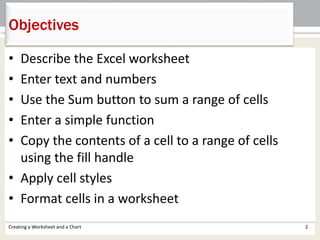
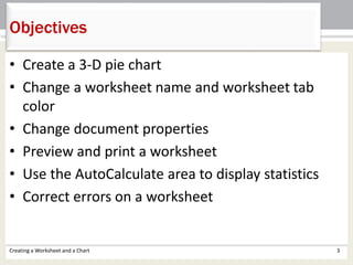
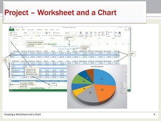
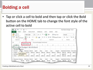
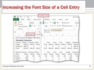
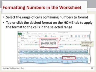
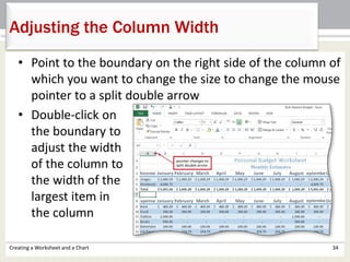
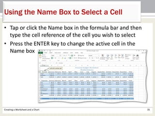
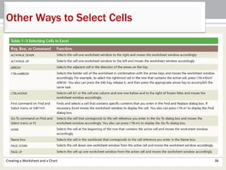
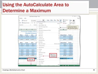
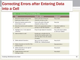
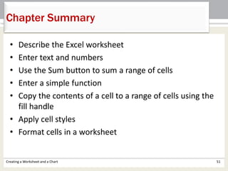
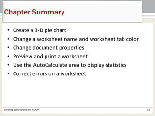
1. Microsoft
Excel 2013
Chapter 1
Creating a Worksheet and
a Chart

2. • Describe the Excel worksheet
• Enter text and numbers
• Use the Sum button to sum a range of cells
• Enter a simple function
• Copy the contents of a cell to a range of cells
using the fill handle
• Apply cell styles
• Format cells in a worksheet
Objectives
Creating a Worksheet and a Chart 2

3. • Create a 3-D pie chart
• Change a worksheet name and worksheet tab
color
• Change document properties
• Preview and print a worksheet
• Use the AutoCalculate area to display statistics
• Correct errors on a worksheet
Creating a Worksheet and a Chart 3
Objectives

4. Creating a Worksheet and a Chart 4
Project – Worksheet and a Chart

5. • Enter text in a blank worksheet
• Calculate sums and use formulas in the worksheet
• Save the workbook using a file name
• Format text in the worksheet
• Insert a pie chart into the worksheet
• Assign a name to the worksheet tab
• Preview and print the worksheet
Creating a Worksheet and a Chart 5
Roadmap

6. Creating a Worksheet and a Chart 6
Entering Worksheet Titles
• Tap or click cell A1 and enter a title for the worksheet
• Tap or click
cell A2 and
enter a
subtitle
• Tap or click
the Enter
box to
complete
the entry

7. Creating a Worksheet and a Chart 7
Entering Column Titles
• Tap or click cell A3 and enter a column title
• Tap cell B3 or press the RIGHT ARROW key to
enter a column title and make the cell to the
right the active cell
• Repeat the previous steps until all column titles
are entered. Click the Enter box after entering
the last column title

8. Creating a Worksheet and a Chart 8
Entering Column Titles

9. Creating a Worksheet and a Chart 9
Entering Row Titles
• Tap or click cell A4 and enter a row title
• Tap cell A5 or press the DOWN ARROW key to
enter a row title and make the cell below the
current cell the active cell
• Repeat the previous steps until all row titles are
entered

10. Creating a Worksheet and a Chart 10
Entering Row Titles

11. Creating a Worksheet and a Chart 11
Entering Numbers
• In Excel, you can enter numbers in Excel to represent amounts
• If a cell entry contains any other keyboard character, Excel
interprets it as
text and treats
it accordingly

12. • Tap or click the first empty cell below the column
of numbers to sum
• Tap or click the Sum button on the HOME tab to
display a formula in the formula bar and in the
active cell
• Tap or click the Enter box in the formula bar to
enter a sum in the active cell
• Repeat above steps to enter the SUM function in
other locations
Creating a Worksheet and a Chart 12
Summing a Column of Numbers

13. Creating a Worksheet and a Chart 13
Summing a Column of Numbers

14. Creating a Worksheet and a Chart 14
Copying a Cell to Adjacent Cells in a Row
• With the cell containing the contents to fill across the
row active, tap AutoFill on the mini toolbar or point to
the fill handle to activate it
• Drag the fill handle to select the destination area to
display a shaded border around the source area and
the destination area
• Lift your finger from the screen or release the mouse
button to copy the SUM function from the active cell
to the destination area and calculate the sums
• Repeat the above steps to copy the SUM function to
other ranges

15. Creating a Worksheet and a Chart 15
Copying a Cell to Adjacent Cells in a Row

16. Creating a Worksheet and a Chart 16
Determining Multiple Totals at the
Same Time
• Highlight a range at the end of rows or
columns of numbers to total
• Tap or click the Sum button on the HOME tab
to calculate and display the sums of the
corresponding rows
• Repeat the above steps to calculate and display
the sums of the corresponding rows

17. Creating a Worksheet and a Chart 17
Determining Multiple Totals at the
Same Time

18. Creating a Worksheet and a Chart 18
Entering a Formula Using the Keyboard
• Select the cell that will contain the formula
• Type the formula in the cell to display it in the
formula bar and in the current cell and to
display colored borders around the cells
referenced in the formula
• Tap or click the cell to the right to complete
the formula and to display the result in the
worksheet.

19. Creating a Worksheet and a Chart 19
Entering a Formula Using the Keyboard

20. Creating a Worksheet and a Chart 20
Formatting the Worksheet
Unformatted
Worksheet
Formatted Worksheet

21. • Tap or click the desired cell and then tap or click
the Cell Styles button on the HOME tab to display
the Cell Styles gallery
• Point to the Title cell style in the Titles and
Headings area of the Cell Styles gallery to see a
live preview of the cell style in the active cell
• Tap or click the Title cell style to apply the cell
style to the active cell
Creating a Worksheet and a Chart 21
Changing a Cell Style

22. Creating a Worksheet and a Chart 22
Changing a Cell Style

23. • Tap or click the desired cell for which you want to
change the font
• Tap or click the Font arrow on the HOME tab to
display the font gallery
• Point to desired font in the Font gallery to see a
live preview of the selected font in the active cell
• Tap or click the desired font to change the font of
the selected cell
Creating a Worksheet and a Chart 23
Changing a Font

24. Creating a Worksheet and a Chart 24
Changing a Font

25. • Tap or click a cell to bold and then tap or click the Bold
button on the HOME tab to change the font style of the
active cell to bold
Creating a Worksheet and a Chart 25
Bolding a cell

26. • With the desired cell selected, tap or click the Font Size
arrow on the HOME tab to display the Font Size gallery
• Point to the desired font size in the Font Size gallery to
see a live preview of the active cell with the selected font
size
• Tap or click the desired font size in the Font Size gallery to
change the font size in the active cell
Creating a Worksheet and a Chart 26
Increasing the Font Size of a Cell Entry

27. Creating a Worksheet and a Chart 27
Increasing the Font Size of a Cell Entry

28. • Select the cell for which you want to change the
font color and then tap or click the Font Color
arrow on the HOME tab
• Point to the desired color in the Theme Colors
area of the Font Color gallery to see a live preview
of the font color
• Tap or click the desired theme to change the font
color of the in the active cell
Creating a Worksheet and a Chart 28
Changing the Font Color of a Cell Entry

29. Creating a Worksheet and a Chart 29
Changing the Font Color of a Cell Entry

30. • Drag to select the range of cells you want to merge and
center
• Tap or click the ‘Merge & Center’ button on the HOME
tab to merge the selected range and center the
contents of the leftmost
cell across the
selected columns
• Repeat the above steps
to merge and center
other titles
Creating a Worksheet and a Chart 30
Centering Cell Entries across Columns by
Merging Cells

31. • Tap or click a cell and drag to select the desired
range
• Tap or click the Cell Styles button on the HOME
tab to display the Cell Styles gallery
• Tap or click a Heading cell style to apply the cell
style to the selected range and then tap or click
the Center button on the HOME tab to center the
column headings in the selected range
• Repeat the above steps to format other ranges
Creating a Worksheet and a Chart 31
Formatting Rows Using Cell Styles

32. Creating a Worksheet and a Chart 32
Formatting Rows Using Cell Styles

33. • Select the range of cells containing numbers to format
• Tap or click the desired format on the HOME tab to apply
the format to the cells in the selected range
Creating a Worksheet and a Chart 33
Formatting Numbers in the Worksheet

34. • Point to the boundary on the right side of the column of
which you want to change the size to change the mouse
pointer to a split double arrow
• Double-click on
the boundary to
adjust the width
of the column to
the width of the
largest item in
the column
Creating a Worksheet and a Chart 34
Adjusting the Column Width

35. • Tap or click the Name box in the formula bar and then
type the cell reference of the cell you wish to select
• Press the ENTER key to change the active cell in the
Name box
Creating a Worksheet and a Chart 35
Using the Name Box to Select a Cell

36. Creating a Worksheet and a Chart 36
Other Ways to Select Cells

37. • Select the range for the 3-D pie chart
• Tap or click the ‘Insert Pie or Doughnut Chart’
button on the INSERT tab to display the Insert Pie or
Doughnut Chart gallery
• Tap or click the Insert Pie or Doughnut Chart gallery
to insert the chart
• Tap or click the chart title to select it
• Type a chart title and then press the ENTER key to
change the title
• Deselect the chart title
Creating a Worksheet and a Chart 37
Adding a 3D Pie Chart

38. Creating a Worksheet and a Chart 38
Adding a 3D Pie Chart

39. • Tap or click the Chart Styles button to display the Chart
Styles gallery
• Tap or click a style in the Chart Styles gallery to change
the chart
style to
the desired
style
Creating a Worksheet and a Chart 39
Applying a Style to a Chart

40. • Tap or click the Move Chart button on the CHART TOOLS
DESIGN tab
• Tap or click New sheet to select it and then type a title for
the worksheet that will contain the chart
• Tap or click the OK button to move the chart to a new
chart sheet with a new sheet tab name
Creating a Worksheet and a Chart 40
Moving a Chart to a New Sheet

41. Creating a Worksheet and a Chart 41
Moving a Chart to a New Sheet

42. Creating a Worksheet and a Chart 42
Changing the Worksheet Tab Name
• Double-tap or double-click the sheet tab you wish
to change in the lower-left corner of the window
• Type a new name as the worksheet tab name
• Press and hold the renamed sheet tab to
display a shortcut menu
• Tap or point to Tab Color in the Tab Color gallery
• Tap or click the desired color in the Theme Colors
area to change the color of the tab

43. Creating a Worksheet and a Chart 43
Changing the Worksheet Tab Name

44. Creating a Worksheet and a Chart 44
Previewing and Printing a Worksheet in
Landscape Orientation
• In Backstage view, tap or click the Print tab to display the
Print gallery
• Verify that the printer listed on the Printer Status button
will print a hard copy of the workbook. If necessary, click
the Printer Status button to display a list of available
printer options and then click the desired printer to
change the currently selected printer
• Tap or click the Portrait Orientation button in the Settings
area and then select Landscape Orientation to change
the orientation of the page to landscape.

45. • Tap or click the No Scaling button and then select
‘Fit Sheet on One Page’ to print the entire
worksheet on one page
• Click the Print button in the Print gallery to print
the worksheet in landscape orientation on the
currently selected printer
• When the printer stops, retrieve the hard copy
Creating a Worksheet and a Chart 45
Previewing and Printing a Worksheet in
Landscape Orientation

46. Creating a Worksheet and a Chart 46
Previewing and Printing a Worksheet in
Landscape Orientation

47. Creating a Worksheet and a Chart 47
Using Common Status Bar Commands

48. • Select the range of which you wish to determine a
maximum, and then press and hold or right-click
the status bar to display the Customize Status Bar
shortcut menu
• Tap or click Maximum on the shortcut menu to
display the Maximum value in the range in the
AutoCalculate area of the status bar
Creating a Worksheet and a Chart 48
Using the AutoCalculate Area to
Determine a Maximum

49. Creating a Worksheet and a Chart 49
Using the AutoCalculate Area to
Determine a Maximum

50. Creating a Worksheet and a Chart 50
Correcting Errors after Entering Data
into a Cell

51. Chapter Summary
Creating a Worksheet and a Chart 51
• Describe the Excel worksheet
• Enter text and numbers
• Use the Sum button to sum a range of cells
• Enter a simple function
• Copy the contents of a cell to a range of cells using the
fill handle
• Apply cell styles
• Format cells in a worksheet

52. Chapter Summary
Creating a Worksheet and a Chart 52
• Create a 3-D pie chart
• Change a worksheet name and worksheet tab color
• Change document properties
• Preview and print a worksheet
• Use the AutoCalculate area to display statistics
• Correct errors on a worksheet

53. Chapter 1 Complete
Microsoft
Excel 2013