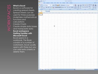
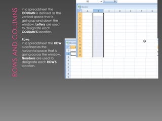
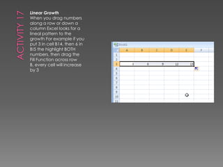
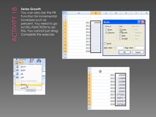
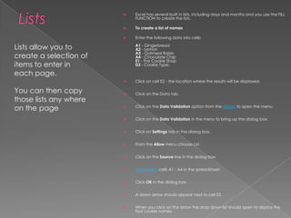
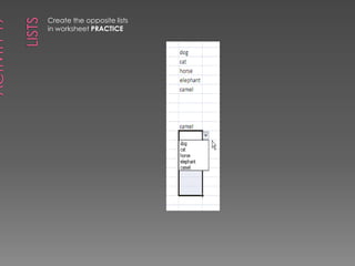
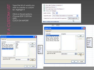
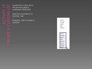
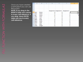
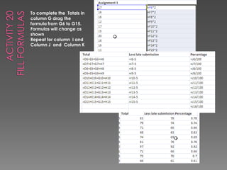
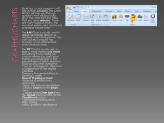
ExcelActivities
WorkSpacesWhat is ExcelExcel is a software for creating spread sheets. Spread sheets can be used for three purposesUndertake mathematical functions and calculationsCreate ChartsCreate simple data bases and manipulate dataExcel workspaceGetting Familiar with Microsoft ExcelExcel opens in a workbook. The Book consists of a number of worksheets. Excel usually opens with three but you can add extra sheets or delete them.
WorksheetsYou can also name each worksheet by double clicking on the worksheet name at the bottom of the page and highlighting it. You can then type in a name. (Or right click on the name and click on RENAME)
Activity 1
Rows and ColumnsIn a spreadsheet the COLUMN is defined as the vertical space that is going up and down the window. Letters are used to designate each COLUMN'S location. RowsIn a spreadsheet the ROW is defined as the horizontal space that is going across the window. Numbers are used to designate each ROW'S location.
CellsCellsIn a spreadsheet the CELL is defined as the space where a specified row and column intersect. Each CELL is assigned a name according to its COLUMN letter and ROW number. In the diagram the CELL labeled B6 is highlighted. When referencing a cell, you should put the column first and the row second. You can see the reference on the top left side of the screen under the toolbars.You move through the cells by clicking on the cell.
HighlightingHighlighting (creating a range)A range is a rectangular block of cells. Many things are accomplished in Excel using ranges. For instance, the format used to display values can be changed for an entire range. A range of cells can also be protected, which means the contents of the cells cannot be altered. Ranges can also be named.
To highlightA single cellClick the cell, or press the arrow keys to move to the cell.A range of cellsClick the first cell of the range, and then drag to the last cell. Click the first cell. Press the F8 key. This anchors the cursor. Note that EXT appears on the Status bar in the lower right corner of the screen. You are in the Extend mode. Click in last cell should now be highlighted. Click esc to finishA large range of cellsClick the first cell in the range, and then hold down SHIFT and click the last cell in the range. You can scroll to make the last cell visible. All cells on a worksheetClick the EDIT SELECT ALL button. Or CONTROL ANonadjacent cells or cell rangesSelect the first cell or range of cells, and then hold down CTRL and select the other cells or ranges.An entire row or columnClick the row or column heading. Adjacent rows or columnsDrag across the row or column headings. Or select the first row or column; then hold down SHIFT and select the last row or column.Nonadjacent rows or columnsSelect the first row or column, and then hold down CTRL and select the other rows or columns.More or fewer cells than the active selectionHold down SHIFT and click the last cell you want to include in the new selection. The rectangular range between the active cell and the cell you click becomes the new selection.Cancel a selection of cellsClick any cell on the worksheet
Activity 2:Highlighting
Shortcuts
SHORT CUTS
Activity 3
EXCEL OPTIONSYou can change the way your Excel Sheet operates through Excel options.Click on the Microsoft buttonEXCEL OPTIONS is on the bottom right hand corner
EXCEL OPTIONSChanges to View , the way the cursor works and layout can all be made through EXCEL OPTIONS
EXCEL OPTIONS
Activity 4
Entering DataIn a spreadsheet there are three basic types of data that can be entered.  LABELS CONSTANTS FORMULAEwe use labels to help identify what we are talking about. The labels are NOT for the computer but rather for US so we can clarify what we are doing. We use them in spread sheets used to calculate formulae’s and databases and to set labels in chartsConstants are entries that have a specific fixed value. In the example: the constants are 40,70,60, 15,10,12. Constants may be different types of numbers. Sometimes constants are referring to dollars, sometimes referring to percentages, and other times referring to a number of items.
Formula Barthe cell address displays on the left side of the Formula bar. Cell entries display on the right side of the Formula bar.‘This display can be text or formulaeIf the display is a formulae the cell will display the result of the formula, the forumlaebar will display the formulae itself.Formula always start with = New lines can be added to the formula bar by using ALT/ENTER
Activity 5Entering text
Entering Numbers If you have a numeric keypad, pressing the Num Lock key can make data entry easier. Num Lock enables you to enter numbers as if you were using a calculator. You can also use the Enter key located on the numeric keypad. If you highlight the rows and columns into which you are going to enter data, the cursor will automatically move up and down those columns.
Activity 6Entering Numbers
Inserting RowsYou can insert or delete rows on the worksheet. You need to insert three rows so you can add headings to the widgets worksheet so it will look like the picture on the right.
Activity 7Inserting Rows
Editing a Cell After you enter data into a cell, you can edit it in the cell as long as you have turned this option on in EXCEL OPTIONS.You can also edit the cell within the Formula bar.
Activity 8Working with Long Text Whenever you type text that is too long to fit into a cell, Microsoft Excel attempts to display all of the text in the next cell. However  if the next cell contains text the cells that contain entries will cut off the long text.
Entering formulasClicking on the cellsInstead of typing in the cell reference it is more accurate to click on the cell.
Activity 9Type in the following data to the work sheet  formula
Activity 10
Activity 11Clicking on CellsClicking on the cellsInstead of typing in the cell reference it is more accurate to click on the cell.
The AutoSum IconT he AutoSum icon on the Standard toolbar automatically creates a SUM function for consecutive numbers, provided there is no ‘empty’ row or column between the numbers The following illustrates using the SUM function to total the Widget SalesWhen you want to add up consecutive numbers, it is much more efficient to use a SUM function than to keep using the + sign.   To add up every cell in Row 5 from column A to D from we could type =A5+B5+C5+D6. It is more efficient to type =SUM(A5:D6). To add every cell in Column A from row 2 to 4 we could type =A2+A3+A4. It is more efficient to type =SUM(A2:A4)
Activity 12 Auto sum
Activity  13Subtraction
Activity 14MultiplicationMultiplicationYou use the * key to indicate multiplication. If Assignment 3 is worth TWICE as many Marks we need to multiply Column F by 2.Multiply each person’s marks for assignment 3 by 2.Go back and change the Total  for Jane Brown for the assignment so it reads
Assignment 15DivisionFor Division we use the / signTo work out the percentage mark divide column J by 100For Jane brown  divide J6/100
Activity 16Fill FunctionExcel can repeat words figures and formulae in a cell Using Fill Function. This means writing headings such as months, repeating formulas and repeating lists are all very easy. You use fill function by dragging the words you want across consecutive cells.Fill function with words.
Activity 17Linear GrowthWhen you drag numbers along a row or down a column Excel looks for a lineal pattern to the growth For example if you put 3 in cell B14, then 6 in B!5 the highlight BOTH numbers, then drag the Fill Function across row B, every cell will increase by 3
Activity 18Series GrowthYou can also Use the Fill Function for incremental increases such as percent. You need to go to\FILL FUNCTION to do this. You cannot just drag.Complete this exercise
ListsExcel has several built in lists, including days and months and you use the FILL FUNCTION to create the lists.To create a list of namesEnter the following data into cells:A1 - Gingerbread A2 - LemonA3 - Oatmeal Raisin A4 - Chocolate ChipE1 - The Cookie Shop D2 - Cookie Type:Click on cell E2 - the location where the results will be displayed.Click on the Data tab.Click on the Data Validation option from the ribbon to open the menu.Click on the Data Validation in the menu to bring up the dialog box.Click on Settings tab in the dialog box.From the Allow menu choose List.Click on the Source line in the dialog box.Drag select cells A1 - A4 in the spreadsheet. Click OK in the dialog box.A down arrow should appear next to cell E2.When you click on the arrow the drop down list should open to display the four cookie names.Lists allow you to create a selection of items to enter in each page.You can then copy those lists any where on the page
Activity 19ListsCreate the opposite lists in worksheet PRACTICE
Create a custom listType the list of words you wish to create a custom list. Highlight itClick on Excel options.Choose EDIT CUSTOM LISTSCLICK ON IMPORT
ACTIVITY 19Create a custom listCreate the custom list in the previous slide in worksheet  PRACTICEType the word lemon in another  cellDrag the  cell to create a word list
Fill Function with FormulasOnce you have created a formulae if you can use fill function.NOTE: If you drag to the RIGHT it adds one column to every cell reference. If you drag  down EXCEL adds one row to every cell reference.
Activity 20Fill formulas To complete the  Totals in  column G drag the formula from G6 to G15.Formulas will change as shownRepeat for column  I and Column J  and  Column K
ReferencingWhen we are entering formulas into a spreadsheet we want to make as many references as possible to other cells because if we can reference that information we don't have to type it in again. AND if  OTHER information changes, we DO-NOT have to change ALL the equations.When we are entering formulas into a spreadsheet we want to make as many references as possible to other cells because if we can reference that information we don't have to type it in again. AND that OTHER information changes, we DO-NOT have to change ALL the equations. In our formula we multiplied everything in Assignment 3 by 2 (g column) and subtracted the scores by 5. It would be better and more practical design if we use a cell Referenced rather than used the figures 2Instead of multiplying everything in Assignment 3 (F Column) by 2 (F column) we should type the figure 2 in cell F3 and then in the F column multiply by the figure in the E column by cell F3 .
Activity 21ReferencingType the figure 2 In G3Type F6*G3 in Cell G3Hit Enter then drag that column downSomething will not be right !!!!!
Activity 22Absolute ValuesWe have already learnt that when you use the fill function and drag downward all formulae cell references change by ONE row (and One Column when you drag across)To FixIn this case you do not want to the formulae to change by one row or column. We always want to multiply from CELL G3 we still want to use the FILL FUNCTION.  The solution is to make those cells ABSOLUTE VALUES. We do this by putting $ signs around any values we do not want to change when we use fill functions.Put a $ sign around G3 in G6 then dragYou will see the F value changes but the G one does not.
Activity 23Pasting absolute valuesSometimes when we enter a formula, we need to repeat the same formula for many different cells. In the spreadsheet we can use the copy and paste command. THE CELL LOCATIONS IN THE FORMULA ARE PASTED RELATIVE TO THE POSITION WE COPY THEM FROM. NOTE: If you COPY a formula with an absolute Value, the absolute value will NOT change. If you CUT a formula with a an ABSOLUTE value, the formula WILL change
Formatting Merging cellsCellsIn Excel regardless of how many cells you want changed. You must Highlight them and use either Icons in format tool bar or FORMAT CELLS Merge cellCentring Across CellsNumbersToolbars. Percentage, Dollar signs Decimal NumbersToolbars. Percentage, Dollar signs Decimal
FormattingColumns/RowsA question that everyone (who has ever worked on a spreadsheet) has asked at one time or another is, "Where did all my numbers go?" or same question, "Where did all of those ####### come from and why are they in my spreadsheet?" The problem is the number trying to be displayed in a particular cell does not have enough width to display properly. To clear up the problem we just need to make the column wider. You can do this many ways. Here are two ways to change the column width Select the column (or columns) with the problem by clicking on their labels (letters). Then you choose the MENU FORMAT. Go down to COLUMN and over to WIDTH and type in a new number for the column width. Move the arrow to the right side of the column label and click and drag the mouse to the right (to make wider) or left (to make smaller). Let up on the mouse button when the column is wide enough. Notice the cursor changes to a vertical line with arrows pointing left and right.Or go to EDIT columns, or EDIT rows and type in the width and height (Columns used characters e.g 1= 1character. Rows use points
Alignment and Border
Activity 23FormattingIN the excel exercises you have done, practice formatting the cellsUse bold
Change angle of text alignments
Change the number formatting and the date
Merge cells and put a heading
Add borders
Colour cellsConditional
Activity 24Format the cells in Formula so that marks below 10 are highlighted in red
Data basesActivity 25Excel has data Base functions. To Create a data base you type your headings then add your data. In this exercise we are going to track the reading skills of 3 classes of childrenNOTE: It is STRONGLY recommended that you always copy a data base to work on it and leave the original intact just in case anything goes wrong.Copy the data base in activities to your worksheetData basesExcel has data Base functions. To Create a data base you type your headings then add your data. In this exercise we are going to track the reading skills of 3 classes of children 
Activity 26Sort If you want to selectively look at data you can use a filter which allows you to see data by different headings.
Activity 27FilterFilter all the classes by number.Then unfilter them
Simple FunctionsMicrosoft Excel has a set of prewritten formulas called functions. Functions differ from regular formulas in that you supply the value but not the operators, such as +, -, *, or /. Use an equals sign to begin a formula Specify the function name Enclose arguments within parentheses Use a comma to separate arguments SumThe SUM function is used to calculate sums. When using a function, remember the following: Here is an example of a function: =SUM(2,13,10,67)The equals sign begins the function SUM is the name of the function 2, 13, 10 and 67 are the arguments Parentheses enclose the arguments A comma separates each of the arguments The SUM function adds the arguments together. It is very useful to use this instead of AutoSum when the cells you want to add up are not together.
Activity 28Average Minimum MaximumCalculating an Average You can use the AVERAGE function to calculate an average from a series of numbers. Calculating Minimum You can use the MIN function to find the lowest number in a series of numbers.
Activity 29 What day were you born
Graphs/ChartsExcel has a chart program built into its main program. The Chart Wizard will step you through questions that will (basically) draw the chart from the data that you have selected. There are many types of charts. The two most widely used are the bar chart and the pie chart. The BAR Chart is usually used to display a change (growth or decline) over a time period. You can quickly compare the numbers of two different bar charts to each other.The PIE Chart is usually used to look at what makes up a wholeSomething. If you had a pie chart of where you spent your money you could look at the percentages of dollars spent on food (or any other category). You can add legends, titles, and change many of the display variables.There are five general steps in defining a chart. Steps in Creating a Chart:Enter the numbers into a workbook.
Select the data to be charted.
Choose Chart from the Insert menu.

Excel

  • 1.
  • 2.
    WorkSpacesWhat is ExcelExcelis a software for creating spread sheets. Spread sheets can be used for three purposesUndertake mathematical functions and calculationsCreate ChartsCreate simple data bases and manipulate dataExcel workspaceGetting Familiar with Microsoft ExcelExcel opens in a workbook. The Book consists of a number of worksheets. Excel usually opens with three but you can add extra sheets or delete them.
  • 3.
    WorksheetsYou can alsoname each worksheet by double clicking on the worksheet name at the bottom of the page and highlighting it. You can then type in a name. (Or right click on the name and click on RENAME)
  • 4.
  • 5.
    Rows and ColumnsIna spreadsheet the COLUMN is defined as the vertical space that is going up and down the window. Letters are used to designate each COLUMN'S location. RowsIn a spreadsheet the ROW is defined as the horizontal space that is going across the window. Numbers are used to designate each ROW'S location.
  • 6.
    CellsCellsIn a spreadsheetthe CELL is defined as the space where a specified row and column intersect. Each CELL is assigned a name according to its COLUMN letter and ROW number. In the diagram the CELL labeled B6 is highlighted. When referencing a cell, you should put the column first and the row second. You can see the reference on the top left side of the screen under the toolbars.You move through the cells by clicking on the cell.
  • 7.
    HighlightingHighlighting (creating arange)A range is a rectangular block of cells. Many things are accomplished in Excel using ranges. For instance, the format used to display values can be changed for an entire range. A range of cells can also be protected, which means the contents of the cells cannot be altered. Ranges can also be named.
  • 8.
    To highlightA singlecellClick the cell, or press the arrow keys to move to the cell.A range of cellsClick the first cell of the range, and then drag to the last cell. Click the first cell. Press the F8 key. This anchors the cursor. Note that EXT appears on the Status bar in the lower right corner of the screen. You are in the Extend mode. Click in last cell should now be highlighted. Click esc to finishA large range of cellsClick the first cell in the range, and then hold down SHIFT and click the last cell in the range. You can scroll to make the last cell visible. All cells on a worksheetClick the EDIT SELECT ALL button. Or CONTROL ANonadjacent cells or cell rangesSelect the first cell or range of cells, and then hold down CTRL and select the other cells or ranges.An entire row or columnClick the row or column heading. Adjacent rows or columnsDrag across the row or column headings. Or select the first row or column; then hold down SHIFT and select the last row or column.Nonadjacent rows or columnsSelect the first row or column, and then hold down CTRL and select the other rows or columns.More or fewer cells than the active selectionHold down SHIFT and click the last cell you want to include in the new selection. The rectangular range between the active cell and the cell you click becomes the new selection.Cancel a selection of cellsClick any cell on the worksheet
  • 9.
  • 10.
  • 11.
  • 12.
  • 13.
    EXCEL OPTIONSYou canchange the way your Excel Sheet operates through Excel options.Click on the Microsoft buttonEXCEL OPTIONS is on the bottom right hand corner
  • 14.
    EXCEL OPTIONSChanges toView , the way the cursor works and layout can all be made through EXCEL OPTIONS
  • 15.
  • 16.
  • 17.
    Entering DataIn aspreadsheet there are three basic types of data that can be entered. LABELS CONSTANTS FORMULAEwe use labels to help identify what we are talking about. The labels are NOT for the computer but rather for US so we can clarify what we are doing. We use them in spread sheets used to calculate formulae’s and databases and to set labels in chartsConstants are entries that have a specific fixed value. In the example: the constants are 40,70,60, 15,10,12. Constants may be different types of numbers. Sometimes constants are referring to dollars, sometimes referring to percentages, and other times referring to a number of items.
  • 18.
    Formula Barthe celladdress displays on the left side of the Formula bar. Cell entries display on the right side of the Formula bar.‘This display can be text or formulaeIf the display is a formulae the cell will display the result of the formula, the forumlaebar will display the formulae itself.Formula always start with = New lines can be added to the formula bar by using ALT/ENTER
  • 19.
  • 20.
    Entering Numbers Ifyou have a numeric keypad, pressing the Num Lock key can make data entry easier. Num Lock enables you to enter numbers as if you were using a calculator. You can also use the Enter key located on the numeric keypad. If you highlight the rows and columns into which you are going to enter data, the cursor will automatically move up and down those columns.
  • 21.
  • 22.
    Inserting RowsYou caninsert or delete rows on the worksheet. You need to insert three rows so you can add headings to the widgets worksheet so it will look like the picture on the right.
  • 23.
  • 24.
    Editing a CellAfter you enter data into a cell, you can edit it in the cell as long as you have turned this option on in EXCEL OPTIONS.You can also edit the cell within the Formula bar.
  • 25.
    Activity 8Working withLong Text Whenever you type text that is too long to fit into a cell, Microsoft Excel attempts to display all of the text in the next cell. However if the next cell contains text the cells that contain entries will cut off the long text.
  • 26.
    Entering formulasClicking onthe cellsInstead of typing in the cell reference it is more accurate to click on the cell.
  • 27.
    Activity 9Type inthe following data to the work sheet formula
  • 28.
  • 29.
    Activity 11Clicking onCellsClicking on the cellsInstead of typing in the cell reference it is more accurate to click on the cell.
  • 30.
    The AutoSum IconT heAutoSum icon on the Standard toolbar automatically creates a SUM function for consecutive numbers, provided there is no ‘empty’ row or column between the numbers The following illustrates using the SUM function to total the Widget SalesWhen you want to add up consecutive numbers, it is much more efficient to use a SUM function than to keep using the + sign. To add up every cell in Row 5 from column A to D from we could type =A5+B5+C5+D6. It is more efficient to type =SUM(A5:D6). To add every cell in Column A from row 2 to 4 we could type =A2+A3+A4. It is more efficient to type =SUM(A2:A4)
  • 31.
  • 32.
  • 33.
    Activity 14MultiplicationMultiplicationYou usethe * key to indicate multiplication. If Assignment 3 is worth TWICE as many Marks we need to multiply Column F by 2.Multiply each person’s marks for assignment 3 by 2.Go back and change the Total for Jane Brown for the assignment so it reads
  • 35.
    Assignment 15DivisionFor Divisionwe use the / signTo work out the percentage mark divide column J by 100For Jane brown divide J6/100
  • 36.
    Activity 16Fill FunctionExcelcan repeat words figures and formulae in a cell Using Fill Function. This means writing headings such as months, repeating formulas and repeating lists are all very easy. You use fill function by dragging the words you want across consecutive cells.Fill function with words.
  • 37.
    Activity 17Linear GrowthWhenyou drag numbers along a row or down a column Excel looks for a lineal pattern to the growth For example if you put 3 in cell B14, then 6 in B!5 the highlight BOTH numbers, then drag the Fill Function across row B, every cell will increase by 3
  • 38.
    Activity 18Series GrowthYoucan also Use the Fill Function for incremental increases such as percent. You need to go to\FILL FUNCTION to do this. You cannot just drag.Complete this exercise
  • 39.
    ListsExcel has severalbuilt in lists, including days and months and you use the FILL FUNCTION to create the lists.To create a list of namesEnter the following data into cells:A1 - Gingerbread A2 - LemonA3 - Oatmeal Raisin A4 - Chocolate ChipE1 - The Cookie Shop D2 - Cookie Type:Click on cell E2 - the location where the results will be displayed.Click on the Data tab.Click on the Data Validation option from the ribbon to open the menu.Click on the Data Validation in the menu to bring up the dialog box.Click on Settings tab in the dialog box.From the Allow menu choose List.Click on the Source line in the dialog box.Drag select cells A1 - A4 in the spreadsheet. Click OK in the dialog box.A down arrow should appear next to cell E2.When you click on the arrow the drop down list should open to display the four cookie names.Lists allow you to create a selection of items to enter in each page.You can then copy those lists any where on the page
  • 40.
    Activity 19ListsCreate theopposite lists in worksheet PRACTICE
  • 41.
    Create a customlistType the list of words you wish to create a custom list. Highlight itClick on Excel options.Choose EDIT CUSTOM LISTSCLICK ON IMPORT
  • 42.
    ACTIVITY 19Create acustom listCreate the custom list in the previous slide in worksheet PRACTICEType the word lemon in another cellDrag the cell to create a word list
  • 43.
    Fill Function withFormulasOnce you have created a formulae if you can use fill function.NOTE: If you drag to the RIGHT it adds one column to every cell reference. If you drag down EXCEL adds one row to every cell reference.
  • 44.
    Activity 20Fill formulasTo complete the Totals in column G drag the formula from G6 to G15.Formulas will change as shownRepeat for column I and Column J and Column K
  • 45.
    ReferencingWhen we areentering formulas into a spreadsheet we want to make as many references as possible to other cells because if we can reference that information we don't have to type it in again. AND if OTHER information changes, we DO-NOT have to change ALL the equations.When we are entering formulas into a spreadsheet we want to make as many references as possible to other cells because if we can reference that information we don't have to type it in again. AND that OTHER information changes, we DO-NOT have to change ALL the equations. In our formula we multiplied everything in Assignment 3 by 2 (g column) and subtracted the scores by 5. It would be better and more practical design if we use a cell Referenced rather than used the figures 2Instead of multiplying everything in Assignment 3 (F Column) by 2 (F column) we should type the figure 2 in cell F3 and then in the F column multiply by the figure in the E column by cell F3 .
  • 46.
    Activity 21ReferencingType thefigure 2 In G3Type F6*G3 in Cell G3Hit Enter then drag that column downSomething will not be right !!!!!
  • 47.
    Activity 22Absolute ValuesWehave already learnt that when you use the fill function and drag downward all formulae cell references change by ONE row (and One Column when you drag across)To FixIn this case you do not want to the formulae to change by one row or column. We always want to multiply from CELL G3 we still want to use the FILL FUNCTION. The solution is to make those cells ABSOLUTE VALUES. We do this by putting $ signs around any values we do not want to change when we use fill functions.Put a $ sign around G3 in G6 then dragYou will see the F value changes but the G one does not.
  • 48.
    Activity 23Pasting absolutevaluesSometimes when we enter a formula, we need to repeat the same formula for many different cells. In the spreadsheet we can use the copy and paste command. THE CELL LOCATIONS IN THE FORMULA ARE PASTED RELATIVE TO THE POSITION WE COPY THEM FROM. NOTE: If you COPY a formula with an absolute Value, the absolute value will NOT change. If you CUT a formula with a an ABSOLUTE value, the formula WILL change
  • 49.
    Formatting Merging cellsCellsInExcel regardless of how many cells you want changed. You must Highlight them and use either Icons in format tool bar or FORMAT CELLS Merge cellCentring Across CellsNumbersToolbars. Percentage, Dollar signs Decimal NumbersToolbars. Percentage, Dollar signs Decimal
  • 50.
    FormattingColumns/RowsA question thateveryone (who has ever worked on a spreadsheet) has asked at one time or another is, "Where did all my numbers go?" or same question, "Where did all of those ####### come from and why are they in my spreadsheet?" The problem is the number trying to be displayed in a particular cell does not have enough width to display properly. To clear up the problem we just need to make the column wider. You can do this many ways. Here are two ways to change the column width Select the column (or columns) with the problem by clicking on their labels (letters). Then you choose the MENU FORMAT. Go down to COLUMN and over to WIDTH and type in a new number for the column width. Move the arrow to the right side of the column label and click and drag the mouse to the right (to make wider) or left (to make smaller). Let up on the mouse button when the column is wide enough. Notice the cursor changes to a vertical line with arrows pointing left and right.Or go to EDIT columns, or EDIT rows and type in the width and height (Columns used characters e.g 1= 1character. Rows use points
  • 51.
  • 52.
    Activity 23FormattingIN theexcel exercises you have done, practice formatting the cellsUse bold
  • 53.
    Change angle oftext alignments
  • 54.
    Change the numberformatting and the date
  • 55.
    Merge cells andput a heading
  • 56.
  • 57.
  • 58.
    Activity 24Format thecells in Formula so that marks below 10 are highlighted in red
  • 59.
    Data basesActivity 25Excelhas data Base functions. To Create a data base you type your headings then add your data. In this exercise we are going to track the reading skills of 3 classes of childrenNOTE: It is STRONGLY recommended that you always copy a data base to work on it and leave the original intact just in case anything goes wrong.Copy the data base in activities to your worksheetData basesExcel has data Base functions. To Create a data base you type your headings then add your data. In this exercise we are going to track the reading skills of 3 classes of children 
  • 60.
    Activity 26Sort Ifyou want to selectively look at data you can use a filter which allows you to see data by different headings.
  • 61.
    Activity 27FilterFilter allthe classes by number.Then unfilter them
  • 62.
    Simple FunctionsMicrosoft Excelhas a set of prewritten formulas called functions. Functions differ from regular formulas in that you supply the value but not the operators, such as +, -, *, or /. Use an equals sign to begin a formula Specify the function name Enclose arguments within parentheses Use a comma to separate arguments SumThe SUM function is used to calculate sums. When using a function, remember the following: Here is an example of a function: =SUM(2,13,10,67)The equals sign begins the function SUM is the name of the function 2, 13, 10 and 67 are the arguments Parentheses enclose the arguments A comma separates each of the arguments The SUM function adds the arguments together. It is very useful to use this instead of AutoSum when the cells you want to add up are not together.
  • 63.
    Activity 28Average MinimumMaximumCalculating an Average You can use the AVERAGE function to calculate an average from a series of numbers. Calculating Minimum You can use the MIN function to find the lowest number in a series of numbers.
  • 64.
    Activity 29 Whatday were you born
  • 65.
    Graphs/ChartsExcel has achart program built into its main program. The Chart Wizard will step you through questions that will (basically) draw the chart from the data that you have selected. There are many types of charts. The two most widely used are the bar chart and the pie chart. The BAR Chart is usually used to display a change (growth or decline) over a time period. You can quickly compare the numbers of two different bar charts to each other.The PIE Chart is usually used to look at what makes up a wholeSomething. If you had a pie chart of where you spent your money you could look at the percentages of dollars spent on food (or any other category). You can add legends, titles, and change many of the display variables.There are five general steps in defining a chart. Steps in Creating a Chart:Enter the numbers into a workbook.
  • 66.
    Select the datato be charted.
  • 67.
    Choose Chart fromthe Insert menu.