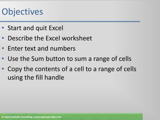
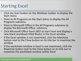
The document outlines the process of creating a worksheet and an embedded chart in Excel, covering objectives such as entering data, formatting cells, summing ranges, and creating 3-D clustered column charts. It includes detailed step-by-step instructions for starting Excel, entering titles and data, applying formatting, saving workbooks, and printing. The guide aims to familiarize users with essential Excel functions and effective worksheet organization.

1. Excel Chapter 1Creating a Worksheet andan Embedded Chart

2. ObjectivesStart and quit ExcelDescribe the Excel worksheetEnter text and numbersUse the Sum button to sum a range of cellsCopy the contents of a cell to a range of cells using the fill handle© OpenCastLabs Consulting. www.opencast-labs.com

3. ObjectivesSave a workbookFormat cells in a worksheetCreate a 3-D Clustered Column chartChange document propertiesSave a workbook a second time using the same file name© OpenCastLabs Consulting. www.opencast-labs.com

4. ObjectivesPrint a worksheetOpen a workbookUse the AutoCalculate area to determine statisticsCorrect errors on a worksheetUse Excel Help to answer questions© OpenCastLabs Consulting. www.opencast-labs.com

5. Plan AheadSelect titles and subtitles for the worksheetDetermine the contents for rows and columnsDetermine the calculations that are neededDetermine where to save the workbookIdentify how to format various elements of the worksheetDecide on the type of chart neededEstablish where to position and how to format the chart© OpenCastLabs Consulting. www.opencast-labs.com

6. Starting ExcelClick the Start button on the Windows taskbar to display the Start menuPoint to All Programs on the Start menu to display the All Programs submenuPoint to Microsoft Office in the All Programs submenu to display the Microsoft Office submenuClick Microsoft Office Excel 2007 to start Excel and display a new blank workbook titled Book1 in the Excel windowIf the Excel window is not maximized, click the Maximize button next to the Close button on its title bar to maximize the windowIf the worksheet window in Excel is not maximized, click the Maximize button next to the Close button on its title bar to maximize the worksheet window within Excel© OpenCastLabs Consulting. www.opencast-labs.com

7. Starting Excel© OpenCastLabs Consulting. www.opencast-labs.com

8. Entering the Worksheet TitlesClick cell A1 to make cell A1 the active cellType Walk and Rock Music in cell A1, and then point to the Enter box in the formula barClick the Enter box to complete the entry and enter the worksheet title in cell A1Click cell A2 to select itType First Quarter Rock-It MP3 Sales as the cell entryClick the Enter box to complete the entry and enter the worksheet subtitle in cell A2© OpenCastLabs Consulting. www.opencast-labs.com

9. Entering the Worksheet Titles© OpenCastLabs Consulting. www.opencast-labs.com

10. Entering Column TitlesClick cell B3 to make cell B3 the active cellType Northeast in cell B3Press the RIGHT ARROW key to enter the column title, Northeast, in cell B3 and make cell C3 the active cellRepeat Steps 2 and 3 to enter the remaining column titles in row 3; that is, enter Southeast in cell C3, Midwest in cell D3, South in cell E3, West in cell F3, and Total in cell G3 (complete the last entry in cell G3 by clicking the Enter box in the formula bar)© OpenCastLabs Consulting. www.opencast-labs.com

11. Entering Column Titles© OpenCastLabs Consulting. www.opencast-labs.com

12. Entering Row TitlesClick cell A4 to select itType Video and then press the DOWN ARROW key to enter the row title and make cell A5 the active cellRepeat Step 1 to enter the remaining row titles in column A; that is, enter Mini in cell A5, Micro in cell A6, Flash in cell A7, Accessories in cell A8, and Total in cell A9© OpenCastLabs Consulting. www.opencast-labs.com

13. Entering Row Titles© OpenCastLabs Consulting. www.opencast-labs.com

14. Entering NumbersClick cell B4Type 66145.15 and then press the RIGHT ARROW key to enter the data in cell B4 and make cell C4 the active cellEnter 79677.1 in cell C4, 34657.66in cell D4, 52517.2 in cell E4, and 99455.49 in cell F4Click cell B5Enter the remaining first quarter sales numbers provided in Table 1–1 on page EX 23 for each of the four remaining offerings in rows 5, 6, 7, and 8 to display the quarterly sales in the worksheet© OpenCastLabs Consulting. www.opencast-labs.com

15. Entering Numbers© OpenCastLabs Consulting. www.opencast-labs.com

16. Summing a Column of NumbersClick cell B9 to make it the active cell and then point to the SUM button on the RibbonClick the Sum button on the Ribbon to display =SUM(B4:B8) in the formula bar and in the active cell B9Click the Enter box in the formula bar to enter the sum of the first quarter sales for the five product types for the Northeast region in cell B9Select cell B9 to display the SUM function assigned to cell B9 in the formula bar© OpenCastLabs Consulting. www.opencast-labs.com

17. Summing a Column of Numbers© OpenCastLabs Consulting. www.opencast-labs.com

18. Copying a Cell to Adjacent Cells in a RowWith cell B9 active, point to the fill handleDrag the fill handle to select the destination area, range C9:F9, to display a shaded border around the destination area, range C9:F9, and the source area, cell B9. Do not release the mouse buttonRelease the mouse button to copy the SUM function in cell B9 to the range C9:F9 and calculate the sums in cells C9, D9, E9, and F9© OpenCastLabs Consulting. www.opencast-labs.com

19. Copying a Cell to Adjacent Cells in a Row© OpenCastLabs Consulting. www.opencast-labs.com

20. Determining Multiple Totals at the Same TimeClick cell G4 to make it the active cellWith the mouse pointer in cell G4 and in the shape of a block plus sign, drag the mouse pointer down to cell G9 to highlight the range G4:G9 with a transparent viewClick the Sum button on the Ribbon to calculate and display the sums of the corresponding rows of sales in cells G4, G5, G6, G7, G8, and G9Select cell A10 to deselect the range G4:G9© OpenCastLabs Consulting. www.opencast-labs.com

21. Determining Multiple Totals at the Same Time© OpenCastLabs Consulting. www.opencast-labs.com

22. Saving a WorkbookWith a USB flash drive connected to one of the computer’s USB ports, click the Save button on the Quick Access Toolbar to display the Save As dialog boxType Walk and Rock Music 1st Quarter Sales in the File name text box to change the file name. Do not press the ENTER key after typing the file nameClick the Save in box arrow to display a list of available drives and foldersClick UDISK 2.0 (E:) in the Save in list to select the USB flash drive, Drive E in this case, as the new save locationClick the Save button in the Save As dialog box to save the workbook on the USB flash drive with the file name, Walk and Rock Music 1st Quarter Sales© OpenCastLabs Consulting. www.opencast-labs.com

23. Saving a Workbook© OpenCastLabs Consulting. www.opencast-labs.com

24. Changing a Cell StyleClick cell A1 to make cell A1 the active cellClick the Cell Styles button on the Ribbon to display the Cell Styles galleryPoint to the Title cell style in the Titles and Headings area of the Cell Styles gallery to see a live preview of the cell style in cell A1Click the Title cell style to apply the cell style to cell A1© OpenCastLabs Consulting. www.opencast-labs.com

25. Changing a Cell Style© OpenCastLabs Consulting. www.opencast-labs.com

26. Changing the Font TypeClick cell A2 to make cell A2 the active cellClick the Font box arrow on the Ribbon to display the Font galleryPoint to Cambria in the Theme Fonts area of the Font gallery to see a live preview of the Cambria font in cell A2Click Cambria in the Theme Fonts area to change the font type of the worksheet subtitle in cell A2 from Calibri to Cambria© OpenCastLabs Consulting. www.opencast-labs.com

27. Changing the Font Type© OpenCastLabs Consulting. www.opencast-labs.com

28. Bolding a CellWith cell A2 active, click the Bold button on the Ribbon to change the font style of the worksheet subtitle to bold© OpenCastLabs Consulting. www.opencast-labs.com

29. Increasing the Font Size of a Cell EntryWith cell A2 selected, click the Font Size box arrow on the Ribbon to display the Font Size listPoint to 14 in the Font Size list to see a live preview of cell A2 with a font size of 14Click 14 in the Font Size list to change the font in cell A2 from 11 point to 14 point© OpenCastLabs Consulting. www.opencast-labs.com

30. Increasing the Font Size of a Cell Entry© OpenCastLabs Consulting. www.opencast-labs.com

31. Changing the Font Color of a Cell EntryWith cell A2 selected, click the Font Color button arrow on the Ribbon to display the Font Color palettePoint to Dark Blue, Text 2 (dark blue color in column 4, row 1) in the Theme Colors area of the Font Color palette to see a live preview of the font color in cell A2Click Dark Blue, Text 2 (column 4, row 1) on the Font Color palette to change the font of the worksheet subtitle in cell A2 from black to dark blue© OpenCastLabs Consulting. www.opencast-labs.com

32. Changing the Font Color of a Cell Entry© OpenCastLabs Consulting. www.opencast-labs.com

33. Centering Cell Entries across Columns by Merging CellsSelect cell A1 and then drag to cell G1 to highlight the range A1:G1Click the Merge and Center button on the Ribbon to merge cells A1 through G1 and center the contents of cell A1 across columns A through GRepeat the first two steps to merge and center the worksheet subtitle across cells A2 through G2© OpenCastLabs Consulting. www.opencast-labs.com

34. Centering Cell Entries across Columns by Merging Cells© OpenCastLabs Consulting. www.opencast-labs.com

35. Formatting Column Titles and the Total RowClick cell A3 and then drag the mouse pointer to cell G3 to select the range A3:G3Point to the Cell Styles button on the RibbonClick the Cell Styles button to display the Cell Styles galleryPoint to the Heading 3 cell style in the Titles and Headings area of the Cell Styles gallery to see a live preview of the cell style in the range A3:G3Click the Heading 3 cell style to apply the cell style to the range A3:G3© OpenCastLabs Consulting. www.opencast-labs.com

36. Formatting Column Titles and the Total RowClick cell A9 and then drag the mouse pointer to cell G9 to select the range A9:G9Point to the Cell Styles button on the RibbonClick the Cell Styles button on the Ribbon to display the Cell Styles gallery and then click the Total cell style in the Titles and Headings area to apply the Total cell style to the cells in the range A9:G9Click cell A11 to select the cell© OpenCastLabs Consulting. www.opencast-labs.com

37. Formatting Column Titles and the Total Row© OpenCastLabs Consulting. www.opencast-labs.com

38. Formatting Numbers in the WorksheetSelect cell B4 and drag the mouse pointer to cell G4 to select the range B4:G4Point to the Accounting Number Format button on the Ribbon to display the Enhanced ScreenTipClick the Accounting Number Format button on the Ribbon to apply the Accounting Number Format to the cells in the range B4:G4Select the range B5:G8© OpenCastLabs Consulting. www.opencast-labs.com

39. Formatting Numbers in the WorksheetClick the Comma Style button on the Ribbon to apply the Comma Style to the range B5:G8Select the range B9:G9Click the Accounting Number Format button on the Ribbon to apply the Accounting Number Format to the cells in the range B9:G9Select cell A11© OpenCastLabs Consulting. www.opencast-labs.com

40. Formatting Numbers in the Worksheet© OpenCastLabs Consulting. www.opencast-labs.com

41. Adjusting Column WidthPoint to the boundary on the right side of the column A heading above row 1 to change the mouse pointer to a split double arrowDouble-click on the boundary to adjust the width of column A to the width of the largest item in the column© OpenCastLabs Consulting. www.opencast-labs.com

42. Adjusting Column Width© OpenCastLabs Consulting. www.opencast-labs.com

43. Using the Name Box to Select a CellClick the Name box in the formula bar and then type a3 as the cell to selectPress the ENTER key to change the active cell from A11 to cell A3© OpenCastLabs Consulting. www.opencast-labs.com

44. Adding a 3-D Clustered Column Chart to the WorksheetClick cell A3 and then drag the mouse pointer to the cell F8 to select the range A3:F8Click the Insert tab to make the Insert tab the active tabClick the Column button on the Ribbon to display the Column galleryPoint to the 3-D Clustered Column chart type in the 3-D Column area of the Column galleryClick the 3-D Clustered Column chart type in the 3-D Column area of the Column gallery to add a 3-D Clustered Column chart to the middle of the worksheet in a selection rectangle© OpenCastLabs Consulting. www.opencast-labs.com

45. Adding a 3-D Clustered Column Chart to the WorksheetClick the top-right edge of the selection rectangle but do not release the mouse to grab the chart and change the mouse pointer to a cross hair with four arrowheadsContinue holding down the left mouse button while dragging the chart down and to the left to position the upper-left corner of the dotted line rectangle over the upper-left corner of cell A11. Release the mouse button to complete the move of the chartClick the middle sizing handle on the right edge of the chart and do not release the mouse buttonWhile continuing to hold down the mouse button, press the ALT key and drag the right edge of the chart to the right edge of column G and then release the mouse button to resize the chartPoint to the middle sizing handle on the bottom edge of the selection rectangle and do not release the mouse button© OpenCastLabs Consulting. www.opencast-labs.com

46. Adding a 3-D Clustered Column Chart to the WorksheetWhile continuing to hold down the mouse button, press the ALT key and drag the bottom edge of the chart up to the bottom edge of row 22 and then release the mouse button to resize the chartClick the More button in the Chart Styles gallery to expand the gallery and point to Style 2 in the gallery (column 2, row 1)Click Style 2 in the Chart Styles gallery to apply the chart style Style 2 to the chartClick cell I9 to deselect the chart and complete the worksheet© OpenCastLabs Consulting. www.opencast-labs.com

47. Adding a 3-D Clustered Column Chart to the Worksheet© OpenCastLabs Consulting. www.opencast-labs.com

48. Changing Document PropertiesClick the Office Button to display the Office Button menuPoint to Prepare on the Office Button menu to display the Prepare submenuClick Properties on the Prepare submenu to display the Document Information PanelClick the Author text box and then type your name as the Author property. If a name already is displayed in the Author text box, delete it before typing your nameClick the Subject text box, if necessary delete any existing text, and then type your course and section as the Subject propertyClick the Keywords text box, if necessary delete any existing text, and then type First Quarter Rock-It MP3 SalesClick the Close the Document Information Panel button so that the Document Information Panel no longer is displayed© OpenCastLabs Consulting. www.opencast-labs.com

49. Changing Document Properties© OpenCastLabs Consulting. www.opencast-labs.com

50. Saving an Existing Workbook with the Same File NameWith your USB flash drive connected to one of the computer’s USB ports, click the Save button on the Quick Access Toolbar to overwrite the previous Walk and Rock Music 1st Quarter Sales file on the USB flash drive© OpenCastLabs Consulting. www.opencast-labs.com

51. Printing a WorksheetClick the Office Button to display the Office button menuPoint to Print on the Office Button menu to display the Print submenuClick Quick Print on the Print submenu to print the document© OpenCastLabs Consulting. www.opencast-labs.com

52. Printing a Worksheet© OpenCastLabs Consulting. www.opencast-labs.com

53. Quitting ExcelPoint to the Close button on the right side of the Excel title barClick the Close button to quit Excel© OpenCastLabs Consulting. www.opencast-labs.com

54. Starting ExcelClick the Start button on the Windows taskbar to display the Start menuPoint to All Programs on the Start menu to display the All Programs submenu and then point to Microsoft Office in the All Programs submenu to display the Microsoft Office submenuClick Microsoft Office Excel 2007 on the Microsoft Office submenu to start Excel and display a new blank worksheet in the Excel windowIf the Excel window is not maximized, click the Maximize button on its title bar to maximize the window© OpenCastLabs Consulting. www.opencast-labs.com

55. Opening a Workbook from ExcelWith your USB flash drive connected to one of the computer’s USB ports, click the Office Button to display the Office Button menuClick Open on the Office Button menu to display the Open dialog boxIf necessary, click the Look in box arrow and then click UDISK 2.0 (E:) to select the USB flash drive, Drive E in this case, in the Look in list as the new open locationClick Walk and Rock Music 1st Quarter Sales to select the file nameClick the Open button to open the selected file and display the worksheet in the Excel window© OpenCastLabs Consulting. www.opencast-labs.com

56. Opening a Workbook from Excel© OpenCastLabs Consulting. www.opencast-labs.com

57. Using the AutoCalculate Area to Determine a MaximumSelect the range B6:F6 and then right-click the AutoCalculate area on the status bar to display the Status Bar Configuration shortcut menuClick Maximum on the shortcut menu to display the Maximum value in the range B6:F6 in the AutoCalculate area of the status barClick anywhere on the worksheet to cause the shortcut menu to disappearRight-click the AutoCalculate area and then click Maximum on the shortcut menu to cause the Maximum value to no longer appear in the AutoCalculate area© OpenCastLabs Consulting. www.opencast-labs.com

58. Using the AutoCalculate Area to Determine a Maximum© OpenCastLabs Consulting. www.opencast-labs.com

59. Searching for Excel HelpClick the Microsoft Office Excel Help button near the upper-right corner of the Excel window to open the Excel Help windowType format a chart in the Type words to search for text box at the top of the Excel Help windowPress the ENTER key to display the search resultsClick the Maximize button on the Excel Help window title bar to maximize the Help windowClick the Format chart elements link to display information regarding formatting chart elementsClick the Close button on the Excel Help window title bar to close the Excel Help window and make Excel active© OpenCastLabs Consulting. www.opencast-labs.com

60. Searching for Excel Help© OpenCastLabs Consulting. www.opencast-labs.com

61. Quitting ExcelClick the Close button on the right side of the title bar to quit ExcelIf necessary, click the No button in the Microsoft Office Excel dialog box so that any changes you have made are not saved© OpenCastLabs Consulting. www.opencast-labs.com

62. SummaryStart and quit ExcelDescribe the Excel worksheetEnter text and numbersUse the Sum button to sum a range of cellsCopy the contents of a cell to a range of cells using the fill handle© OpenCastLabs Consulting. www.opencast-labs.com

63. SummarySave a workbookFormat cells in a worksheetCreate a 3-D Clustered Column chartChange document propertiesSave a workbook a second time using the same file name© OpenCastLabs Consulting. www.opencast-labs.com

64. SummaryPrint a worksheetOpen a workbookUse the AutoCalculate area to determine statisticsCorrect errors on a worksheetUse Excel Help to answer questions© OpenCastLabs Consulting. www.opencast-labs.com

65. Excel Chapter 1 Complete