Download as PDF, PPTX


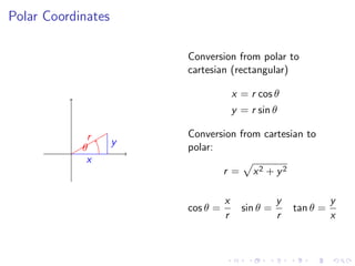
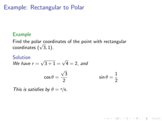

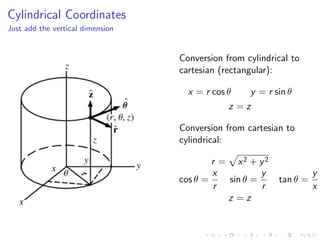

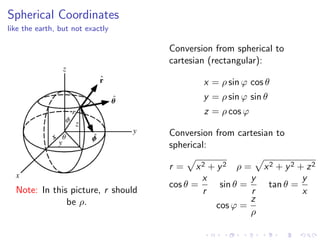
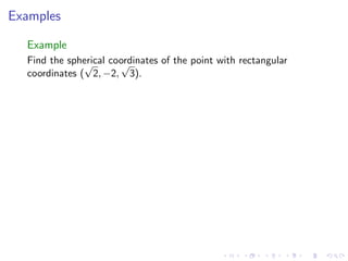
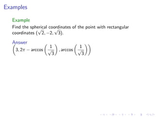
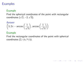


This document outlines various coordinate systems including polar, cylindrical, and spherical coordinates, describing their significance in measuring space. It provides examples of conversions between these coordinate systems and includes specific problems and solutions for clarification. Additionally, it notes the schedule for classes and office hours related to the course on the topic.