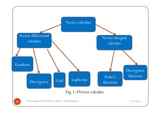
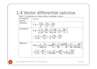
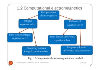
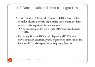
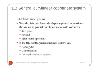
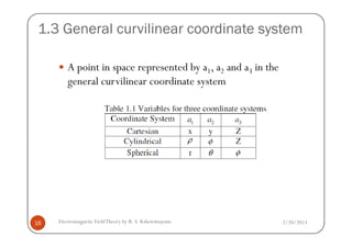
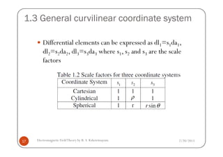
This document discusses electromagnetic field theory and computational electromagnetics. It introduces electromagnetic theory, which is divided into electrostatics, magnetostatics, and time-varying fields. Computational electromagnetics is presented as a way to numerically solve electromagnetic problems using computers. Different types of equation solvers are described, including integral equation solvers and differential equation solvers. General coordinate systems and transformations between coordinate systems are also covered.
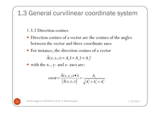
![1.3 General curvilinear coordinate system
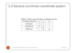
1.3.3 Coordinate transformations
(a) Spherical to Rectangular and vice versa
( ) [ ] ( )
sin cos cos cos sin
sin sin cos sin cos , , , ,
x r
y sr
A A
A A A x y z T A rθ
θ φ θ φ φ
θ φ θ φ φ θ φ
−
= ⇒ =
r r
2/20/2013Electromagnetic FieldTheory by R. S. Kshetrimayum26
( ) [ ] ( )
cos sin 0
y sr
z
AA
θ
φθ θ
−
sin cos sin sin cos
cos cos cos sin sin
sin cos 0
xr
y
z
AA
A A
A A
θ
φ
θ φ θ φ θ
θ φ θ φ θ
φ φ
= −
− ](https://image.slidesharecdn.com/1slides-150503001028-conversion-gate02/85/1-slides-26-320.jpg)
![1.3 General curvilinear coordinate system
(b) Cylindrical to Rectangular and vice versa
( ) [ ] ( )
cos sin 0
sin cos 0 , , , ,
0 0 1
x
y cr
zz
AA
A A A x y z T A z
AA
ρ
φ
φ φ
φ φ ρ φ
−
= ⇒ =
r r
2/20/2013Electromagnetic FieldTheory by R. S. Kshetrimayum27
cos sin 0
sin cos 0
0 0 1
x
y
z z
A A
A A
A A
ρ
φ
φ φ
φ φ
= −
](https://image.slidesharecdn.com/1slides-150503001028-conversion-gate02/85/1-slides-27-320.jpg)
![1.3 General curvilinear coordinate system
(c) Spherical to Cylindrical and vice versa
( ) [ ] ( )
sin cos 0
0 0 1 , , , ,
cos sin 0
r
sc
z
A A
A A A z T A r
AA
ρ
φ θ
φ
θ θ
ρ φ θ φ
θ θ
= ⇒ =
−
r r
2/20/2013Electromagnetic FieldTheory by R. S. Kshetrimayum28
sin 0 cos
cos 0 sin
0 1 0
r
z
AA
A A
A A
ρ
θ φ
φ
θ θ
θ θ
= −
](https://image.slidesharecdn.com/1slides-150503001028-conversion-gate02/85/1-slides-28-320.jpg)