The document discusses various coordinate systems and vector calculus concepts. It defines Cartesian, cylindrical, and spherical coordinate systems. It describes how to write vectors and relationships between components in different coordinate systems. It also covers vector operations like gradient, divergence, curl, and Laplacian as well as line, surface, and volume integrals. Examples are provided to illustrate calculating the gradient of scalar fields defined in different coordinate systems.

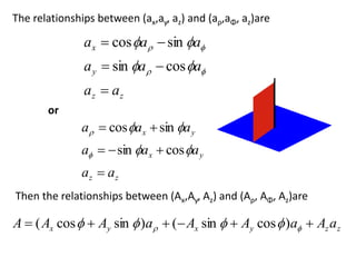
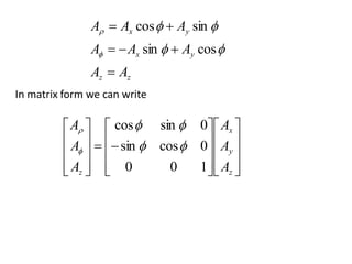
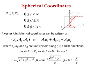
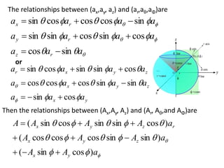
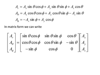
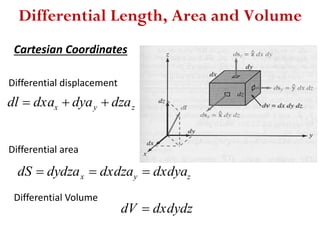
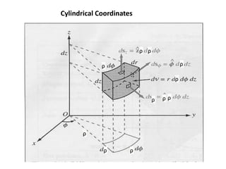
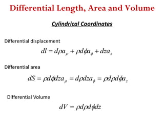
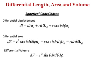
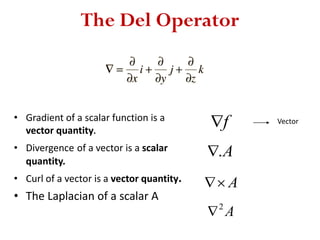
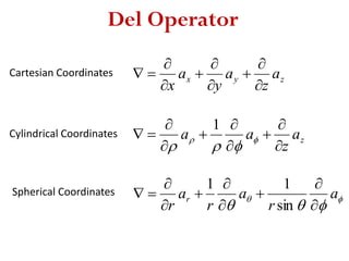
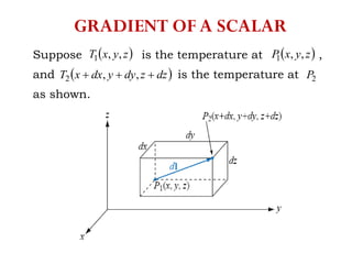
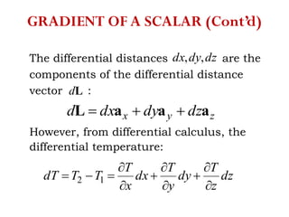
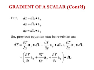
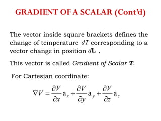
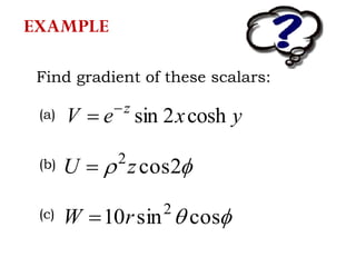
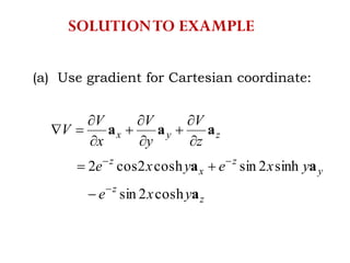
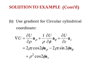
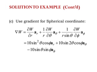
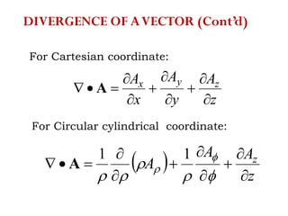
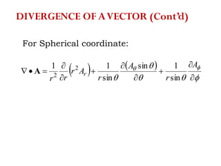
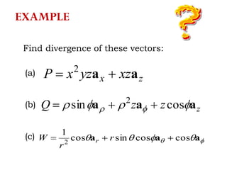
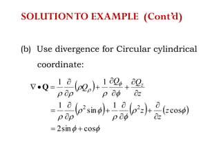
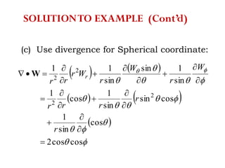
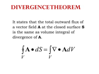
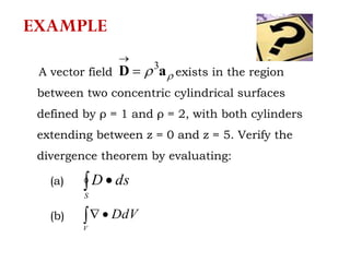
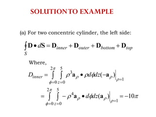
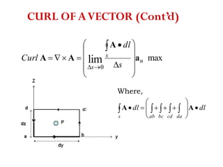
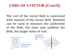
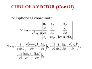
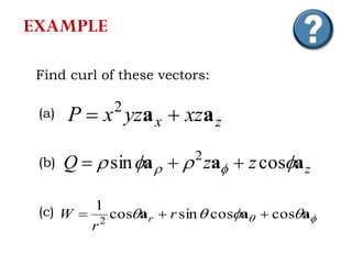
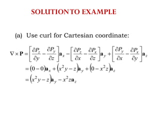
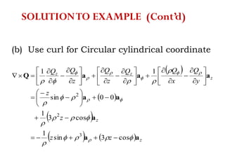
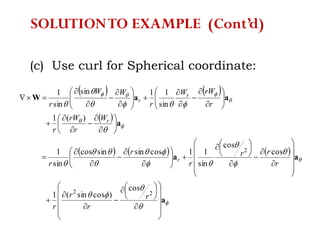
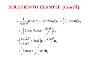
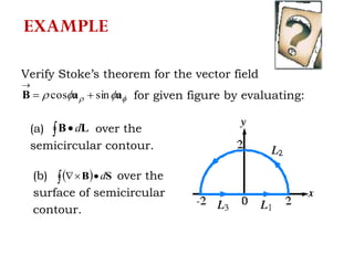
1. Coordinate Systems andTransformations
&
Vector Calculus
By:
Hanish Garg
12105017
ECE Branch
PEC University ofTechnology

2. Coordinate Systems
• Cartesian or Rectangular Coordinate System
• Cylindrical Coordinate System
• Spherical Coordinate System
Choice of the system is based on the symmetry of the
problem.

3. Cartesian Or Rectangular Coordinates
P (x, y, z)
x
y
z
P(x,y,z)



z
y
x
A vector A in Cartesian coordinates can be written as
),,( zyx AAA or zzyyxx aAaAaA 
where ax,ay and az are unit vectors along x, y and z-directions.

4. Cylindrical Coordinates
P (ρ, Φ, z)
x= ρ cos Φ, y=ρ sin Φ, z=z
z
Φ
z
ρ
x
y
P(ρ, Φ, z)



z


20
0
A vector A in Cylindrical coordinates can be written as
),,( zAAA  or
zzaAaAaA  
where aρ,aΦ and az are unit vectors along ρ, Φ and z-directions.
zz
x
y
yx  
,tan, 122


5. The relationships between (ax,ay, az) and (aρ,aΦ, az)are
zz
y
x
aa
aaa
aaa







cossin
sincos
zz
yx
yx
aa
aaa
aaa







cossin
sincos
or
zzyxyx aAaAAaAAA    )cossin()sincos(
Then the relationships between (Ax,Ay, Az) and (Aρ, AΦ, Az)are

6. zz
yx
yx
AA
AAA
AAA







cossin
sincos































z
y
x
z A
A
A
A
A
A
100
0cossin
0sincos




In matrix form we can write

8. Spherical Coordinates
P (r, θ, Φ)
x=r sin θ cos Φ, y=r sin θ sin Φ, Z=r cos θ


20
0
0


 r
A vector A in Spherical coordinates can be written as
),,(  AAAr or  aAaAaA rr 
where ar, aθ, and aΦ are unit vectors along r, θ, and Φ-directions.
θ
Φ
r
z
y
x
P(r, θ, Φ)
x
y
z
yx
zyxr 1
22
1222
tan,tan, 


 

9. The relationships between (ax,ay, az) and (ar,aθ,aΦ)are






aaa
aaaa
aaaa
rz
ry
rx
sincos
cossincossinsin
sincoscoscossin



yx
zyx
zyxr
aaa
aaaa
aaaa





cossin
sinsincoscoscos
cossinsincossin



or
Then the relationships between (Ax,Ay, Az) and (Ar, Aθ,and AΦ)are





aAA
aAAA
aAAAA
yx
zyx
rzyx
)cossin(
)sinsincoscoscos(
)cossinsincossin(




10. 































z
y
xr
A
A
A
A
A
A
0cossin
sinsincoscoscos
cossinsincossin





In matrix form we can write





cossin
sinsincoscoscos
cossinsincossin
yx
zyx
zyxr
AAA
AAAA
AAAA




12. Cartesian Coordinates
P(x, y, z)
Spherical Coordinates
P(r, θ, Φ)
Cylindrical Coordinates
P(ρ, Φ, z)
x
y
z
P(x,y,z)
Φ
z
r
x
y
z
P(ρ, Φ, z)
θ
Φ
r
z
y
x
P(r, θ, Φ)

13. Differential Length, Area and Volume
Differential displacement
zyx dzadyadxadl 
Differential area
zyx dxdyadxdzadydzadS 
Differential Volume
dxdydzdV 
Cartesian Coordinates

14. Cylindrical Coordinates
ρρ
ρ
ρ
ρρ
ρ
ρ
ρρ
ρ

15. Differential Length, Area and Volume
Differential displacement
zdzaadaddl   
Differential area
zadddzaddzaddS   
Differential Volume
dzdddV 
Cylindrical Coordinates

16. Spherical Coordinates

17. Differential Length, Area and Volume
Differential displacement
  adrarddradl r sin
Differential area
  ardrdadrdraddrdS r  sinsin2
Differential Volume
 ddrdrdV sin2

Spherical Coordinates

18. Line, Surface and Volume Integrals
Line Integral
L
dlA.
Surface Integral
Volume Integral

S
dSA.
dvp
V
v

19. • Gradient of a scalar function is a
vector quantity.
• Divergence of a vector is a scalar
quantity.
• Curl of a vector is a vector quantity.
• The Laplacian of a scalar A
f Vector
A.
A
A2

The Del Operator

20. Del Operator
Cartesian Coordinates zyx a
z
a
y
a
x 








Cylindrical Coordinates
Spherical Coordinates
za
z
aa








 

1


a
r
a
r
a
r
r









sin
11

21. VECTOR CALCULUS
GRADIENT OFA SCALAR
DIVERGENCE OFAVECTOR
DIVERGENCETHEOREM
CURL OFAVECTOR
STOKES’STHEOREM

22. GRADIENT OF A SCALAR
Suppose is the temperature at ,
and is the temperature at
as shown.
 zyxT ,,1  zyxP ,,1
2P dzzdyydxxT  ,,2

23. The differential distances are the
components of the differential distance
vector :
dzdydx ,,
zyx dzdydxd aaaL 
Ld
However, from differential calculus, the
differential temperature:
dz
z
T
dy
y
T
dx
x
T
TTdT








 12
GRADIENT OF A SCALAR (Cont’d)

24. But,
z
y
x
ddz
ddy
ddx
aL
aL
aL



So, previous equation can be rewritten as:
Laaa
LaLaLa
d
z
T
y
T
x
T
d
z
T
d
y
T
d
x
T
dT
zyx
zyx

























GRADIENT OF A SCALAR (Cont’d)

25. The vector inside square brackets defines the
change of temperature corresponding to a
vector change in position .
This vector is called Gradient of Scalar T.
Ld
dT
For Cartesian coordinate:
zyx
z
V
y
V
x
V
V aaa









GRADIENT OF A SCALAR (Cont’d)

26. For Circular cylindrical coordinate:
z
z
VVV
V aaa








 

1
For Spherical coordinate:


aaa









V
r
V
rr
V
V r
sin
11
GRADIENT OF A SCALAR (Cont’d)

27. EXAMPLE
Find gradient of these scalars:
yxeV z
cosh2sin

 2cos2
zU 
 cossin10 2
rW 
(a)
(b)
(c)

28. SOLUTIONTO EXAMPLE
(a) Use gradient for Cartesian coordinate:
z
z
y
z
x
z
zyx
yxe
yxeyxe
z
V
y
V
x
V
V
a
aa
aaa
cosh2sin
sinh2sincosh2cos2














29. SOLUTIONTO EXAMPLE (Cont’d)
(b) Use gradient for Circular cylindrical
coordinate:
z
z
zz
z
UUU
U
a
aa
aaa





2cos
2sin22cos2
1
2












30. (c) Use gradient for Spherical coordinate:






a
aa
aaa
sinsin10
cos2sin10cossin10
sin
11
2











r
r
W
r
W
rr
W
W
SOLUTIONTO EXAMPLE (Cont’d)

31. Illustration of the divergence of a vector
field at point P:
Positive
Divergence
Negative
Divergence
Zero
Divergence
DIVERGENCE OF AVECTOR

32. DIVERGENCE OF AVECTOR (Cont’d)
The divergence of A at a given point P
is the outward flux per unit volume:
v
dS
div s
v 




A
AA lim
0

33. What is ?? 
s
dSA Vector field A at
closed surface S
DIVERGENCE OF AVECTOR (Cont’d)

34. Where,
dSdS
bottomtoprightleftbackfronts









  AA
And, v is volume enclosed by surface S
DIVERGENCE OF AVECTOR (Cont’d)

35. For Cartesian coordinate:
z
A
y
A
x
A zyx








 A
For Circular cylindrical coordinate:
  z
AA
A z














11
A
DIVERGENCE OF AVECTOR (Cont’d)

36. For Spherical coordinate:
   













A
r
A
r
Ar
rr
r
sin
1sin
sin
11 2
2
A
DIVERGENCE OF AVECTOR (Cont’d)

37. Find divergence of these vectors:
zx xzyzxP aa  2
zzzQ aaa   cossin 2

  aaa coscossincos
1
2
 r
r
W r
(a)
(b)
(c)
EXAMPLE

38. 39
(a) Use divergence for Cartesian
coordinate:
     
xxyz
xz
zy
yzx
x
z
P
y
P
x
P zyx



















2
02
P
SOLUTIONTO EXAMPLE

39. (b) Use divergence for Circular cylindrical
coordinate:
 
     










cossin2
cos
1
sin
1
11
22


















 Q
z
z
z
z
QQ
Q z
SOLUTIONTO EXAMPLE (Cont’d)

40. (c) Use divergence for Spherical coordinate:
   
   
 










coscos2
cos
sin
1
cossin
sin
1
cos
1
sin
1sin
sin
11
2
2
2
2


















 W
r
r
rrr
W
r
W
r
Wr
rr
r
SOLUTIONTO EXAMPLE (Cont’d)

41. It states that the total outward flux of
a vector field A at the closed surface S
is the same as volume integral of
divergence of A.
 
VV
dVdS AA
DIVERGENCETHEOREM

42. A vector field exists in the region
between two concentric cylindrical surfaces
defined by ρ = 1 and ρ = 2, with both cylinders
extending between z = 0 and z = 5. Verify the
divergence theorem by evaluating:
 aD 3


 
S
dsD
 
V
DdV
(a)
(b)
EXAMPLE

43. (a) For two concentric cylinder, the left side:
topbottomouterinner
S
d DDDDSD 
Where,










10)(
)(
2
0
5
0
1
4
2
0
5
0
1
3


 
 
 

 

z
z
inner
dzd
dzdD
aa
aa
SOLUTIONTO EXAMPLE

44. 









160)(
)(
2
0
5
0
2
4
2
0
5
0
2
3


 
 
 

 

z
z
outer
dzd
dzdD
aa
aa
 
 
 

 



2
1
2
0
5
3
2
1
2
0
0
3
0)(
0)(










z
ztop
z
zbottom
ddD
ddD
aa
aa
SOLUTIONTO EXAMPLE (Cont’d)

45. Therefore


150
0016010

 SD
S
d
SOLUTIONTO EXAMPLE (Cont’d)

46. (b) For the right side of Divergence Theorem,
evaluate divergence of D
  23
4
1





 D
So,





 
150
4
5
0
2
0
2
1
4
5
0
2
0
2
1
2





























  
  
z
r
z
dzdddVD
SOLUTIONTO EXAMPLE (Cont’d)

47. CURL OF AVECTOR
The curl of vector A is an axial
(rotational) vector whose magnitude is
the maximum circulation of A per unit
area tends to zero and whose direction
is the normal direction of the area
when the area is oriented so as to
make the circulation maximum.

48. maxlim
0
a
A
AA n
s
s s
dl
Curl















Where,
CURL OF AVECTOR (Cont’d)
dldl
dacdbcabs








  AA

49. The curl of the vector field is concerned
with rotation of the vector field. Rotation
can be used to measure the uniformity
of the field, the more non uniform the
field, the larger value of curl.
CURL OF AVECTOR (Cont’d)

50. For Cartesian coordinate:
zyx
zyx
AAA
zyx 






aaa
A
z
xy
y
xz
x
yz
y
A
x
A
z
A
x
A
z
A
y
A
aaaA 































CURL OF AVECTOR (Cont’d)

51. z
z
AAA
z





 






aaa
A
1
 
z
zz
AA
z
AA
z
AA
a
aaA












































1
1
For Circular cylindrical coordinate:
CURL OF AVECTOR (Cont’d)

52. For Spherical coordinate:
  



ArrAA
rr
r
r
sin
sin
1
2







aaa
A
   
 








a
aaA



































r
r
r
A
r
rA
r
r
rAA
r
AA
r
)(1
sin
11sin
sin
1
CURL OF AVECTOR (Cont’d)

53. zx xzyzxP aa  2
zzzQ aaa   cossin 2

  aaa coscossincos
1
2
 r
r
W r
(a)
(b)
(c)
Find curl of these vectors:
EXAMPLE

54. (a) Use curl for Cartesian coordinate:
     
  zy
zyx
z
xy
y
xz
x
yz
zxzyx
zxzyx
y
P
x
P
z
P
x
P
z
P
y
P
aa
aaa
aaaP
22
22
000


































SOLUTIONTO EXAMPLE

55. (b) Use curl for Circular cylindrical coordinate
 
 
 
    z
z
z
zz
zz
z
z
y
Q
x
QQ
z
Q
z
QQ
aa
a
aa
aaaQ















cos3sin
1
cos3
1
00sin
11
3
2
2













































SOLUTIONTO EXAMPLE (Cont’d)

56. (c) Use curl for Spherical coordinate:
   
 
     





















a
aa
a
aaW






















































































22
2
cos
)cossin(1
cos
cos
sin
11cossinsincos
sin
1
)(1
sin
11sin
sin
1
r
r
r
r
r
rr
r
r
r
W
r
rW
r
r
rWW
r
WW
r
r
r
r
r
SOLUTIONTO EXAMPLE (Cont’d)

57.    
a
aa
a
aa













sin
1
cos2
cos
sin
sin
2cos
sin
cossin2
1
cos0
1
sinsin2cos
sin
1
3
2






















r
rr
r
r
r
r
r
r
r
r
SOLUTIONTO EXAMPLE (Cont’d)

58. STOKE’STHEOREM
The circulation of a vector field A around
a closed path L is equal to the surface
integral of the curl of A over the open
surface S bounded by L that A and curl
of A are continuous on S.
  
SL
dSdl AA

59. STOKE’STHEOREM (Cont’d)

60. By using Stoke’s Theorem, evaluate
for
  dlA
  aaA sincos 

EXAMPLE

62. Stoke’s Theorem,
  
SL
dSdl AA
where, andzddd aS 
Evaluate right side to get left side,
  zaA 

sin1
1

SOLUTIONTO EXAMPLE (Cont’d)

63.    
941.4
sin1
1
0
0
60
30
5
2

  
 
aA z
S
dddS 
 
SOLUTIONTO EXAMPLE (Cont’d)

64. Verify Stoke’s theorem for the vector field
for given figure by evaluating:  aaB sincos 

(a) over the
semicircular contour.
  LB d
(b) over the
surface of semicircular
contour.
   SB d
EXAMPLE

65. (a) To find  LB d
 
321 LLL
dddd LBLBLBLB
Where,
   

 
dd
dzddd z
sincos
sincos

 aaaaaLB
SOLUTIONTO EXAMPLE

66. So
20
2
1
sincos
2
0
2
0
0
0
0,0
2
01


































LB
zz
L
ddd
  4cos20
sincos
0
0,2
0
0
2
22































LB
zz
L
ddd
SOLUTIONTO EXAMPLE (Cont’d)

67. 20
2
1
sincos
0
2
2
00,0
0
23































r
zz
L
ddd




LB
Therefore the closed integral,
8242  LB d
SOLUTIONTO EXAMPLE (Cont’d)

68. (b) To find    SB d
 
       
   
     
z
z
z
zz
a
aaa
a
aa
aaB



























































1
1sin
sinsin
1
00
cossin
1
0cossin0
1
sincos
SOLUTIONTO EXAMPLE (Cont’d)

69. Therefore
 
8
2
1
cos
1sin
1
1sin
0
2
0
2
0
2
0
0
2
0






































 
 
 
 




 

 




 aaSB
dd
ddd zz
SOLUTIONTO EXAMPLE (Cont’d)

70. LAPLACIAN OF A SCALAR
The Laplacian of a scalar field, V
written as:
V2

Where, Laplacian V is:






























zyxzyx
z
V
y
V
x
V
zyx
VV
aaaaaa
2

71. For Cartesian coordinate:
2
2
2
2
2
2
2
z
V
y
V
x
V
V









For Circular cylindrical coordinate:
2
22
2
2 11
z
VVV
V



















LAPLACIAN OF A SCALAR (Cont’d)

72. LAPLACIAN OF A SCALAR (Cont’d)
For Spherical coordinate:
2
2
22
2
2
2
2
sin
1
sin
sin
11




























V
r
V
rr
V
r
rr
V

73. EXAMPLE
Find Laplacian of these scalars:
yxeV z
cosh2sin

 2cos2
zU 
 cossin10 2
rW 
(a)
(b)
(c)
You should try this!!

74. SOLUTIONTO EXAMPLE
yxeV z
cosh2sin22 

02
 U
 

2cos21
cos102

r
W
(a)
(b)
(c)

75. ThankYou !!!