Downloaded 18 times
![MAT 10B: Highlights
Fall 2011 - Williams
Latest Update: November 22, 2011
Section 5.1. Introduction: Areas and Volumes
Definition (Standard rectangle in R2
). Let a, b, c, d be real numbers such that a < b and
c < d. These numbers determine a closed rectangle
R = {(x, y) | a x b , c y d} ⇢ R2
.
We also denote this rectangle as
R = [a, b] ⇥ [c, d] .
Computational Tool: Iterated integrals
Let R = [a, b] ⇥ [c, d] be a rectangle. Let f : R ! [0, 1) be a continuous function. Then the
integral Z d
c
Z b
a
f(x, y) dx dy
is interpreted as the iterated integral
Z d
c
✓Z b
a
f(x, y) dx
◆
dy .
When computing the “inner integral”
Z b
a
f(x, y) dx ,
treat y as a constant.
Similarly, Z b
a
Z d
c
f(x, y) dy dx =
Z b
a
✓Z d
c
f(x, y) dy
◆
dx .
1](https://image.slidesharecdn.com/notesuptoch7sec3-140410165830-phpapp01/85/Notes-up-to_ch7_sec3-1-320.jpg)
![MAT 10B: Highlights
Fall 2011 - Williams
Latest Update: November 22, 2011
Section 5.1. Introduction: Areas and Volumes
Definition (Standard rectangle in R2
). Let a, b, c, d be real numbers such that a < b and
c < d. These numbers determine a closed rectangle
R = {(x, y) | a x b , c y d} ⇢ R2
.
We also denote this rectangle as
R = [a, b] ⇥ [c, d] .
Computational Tool: Iterated integrals
Let R = [a, b] ⇥ [c, d] be a rectangle. Let f : R ! [0, 1) be a continuous function. Then the
integral Z d
c
Z b
a
f(x, y) dx dy
is interpreted as the iterated integral
Z d
c
✓Z b
a
f(x, y) dx
◆
dy .
When computing the “inner integral”
Z b
a
f(x, y) dx ,
treat y as a constant.
Similarly, Z b
a
Z d
c
f(x, y) dy dx =
Z b
a
✓Z d
c
f(x, y) dy
◆
dx .
1](https://image.slidesharecdn.com/notesuptoch7sec3-140410165830-phpapp01/75/Notes-up-to_ch7_sec3-1-2048.jpg)
![Example.
Z 2
0
Z 3
1
x2
+ y dy dx =
Z 2
0
✓Z 3
1
x2
+ y dy
◆
dx
=
Z 2
0
h
x2
y +
y2
2
iy=3
y=1
dx
=
Z 2
0
✓
3x2
+
9
2
◆ ✓
x2
+
1
2
◆
dx
=
Z 2
0
2x2
+ 4 dx
=
40
3
.
We compute the associated integral in which the order of integration is switched.
Z 3
1
Z 2
0
x2
+ y dx dy =
Z 3
1
✓Z 2
0
x2
+ y dx
◆
dy
=
Z 3
1
hx3
3
+ xy
ix=2
x=0
dy
=
Z 3
1
8
3
+ 2y dy
=
40
3
.
We happen to get the same answer of 40
3
. This is no coincidence since the integral represents
the same geometric quantity; also see Fubini’s Theorem in the next section.
Proposition. Let R = [a, b] ⇥ [c, d] be a rectangle.
Let f : R ! [0, 1) be a continuous function.
If V denotes the volume of the region between the graph of f and the xy–plane, then
V =
Z b
a
Z d
c
f(x, y) dy dx =
Z d
c
Z b
a
f(x, y) dx dy .
A simplified notation for the above iterated integral is
ZZ
R
f dA .
Example (Volume of a box). Suppose that a box has dimensions l, w, h. Draw a picture in
R3
. Then the volume of the box is
V =
Z l
0
Z w
0
h dy dx =
Z l
0
wh dx = lwh .
2](https://image.slidesharecdn.com/notesuptoch7sec3-140410165830-phpapp01/85/Notes-up-to_ch7_sec3-2-320.jpg)
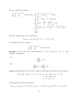
![Example (Volume of a complicated region). Find the volume of the region bounded by the
graph of
f(x, y) = 9 x2
y2
over the rectangle R = [1, 2] ⇥ [0, 1].
The volume is
V =
Z 2
1
Z 1
0
9 x2
y2
dy dx
=
Z 2
1
✓
26
3
x2
◆
dx
=
19
3
.
Section 5.2. Double Integrals
Goals: Define the double integral ZZ
R
f dA
1. for a more general function f : R ! R (not necessarily nonnegative nor continuous)
2. over a more general region R ⇢ R (not necessarily a rectangle).
Part 1: Integral of a function over a rectangle
Definition (Partition of order n). Let R = [a, b] ⇥ [c, d] be a rectangle, and let n be a
positive integer. Consider partitions
a = x0 < x1 < x2 < · · · < xn = b for [a, b], and
c = y0 < y1 < y2 < · · · < yn = d for [c, d].
A partition of order n (of R) is the collection of subrectangles
Rij = [xi 1, xi] ⇥ [yj 1, yj]
for i, j = 1, . . . , n. Visualize the partition as a tiling of R.
Given Rij, the base is xi = xi xi 1 and the height is yj = yj yj 1.
The area of Rij is
Aij = xi · yj .
Furthermore, the partition is called regular if xi = b a
n
and yj = d c
n
for all i, j =
1, . . . , n.
3](https://image.slidesharecdn.com/notesuptoch7sec3-140410165830-phpapp01/85/Notes-up-to_ch7_sec3-3-320.jpg)
![Definition (Riemann Sum). Let R = [a, b] ⇥ [c, d] be a rectangle.
Choose a partition {Rij} for R.
For each i, j = 1, . . . , n, choose a sample point cij 2 Rij.
Let f : R ! R be a function.
The quantity
S =
nX
i,j=1
f(cij) Aij ,
is called a Riemann sum.
Now we give the definition of the double integral.
Definition (Double Integral). Let R = [a, b] ⇥ [c, d] be a rectangle.
Let f : R ! R be a function.
The double integral of f over R is defined to be
ZZ
R
f dA = lim
n!1
nX
i,j=1
f(cij) Aij
over all regular partitions Rij of R.
Remark. The above definition of
RR
R
f dA is equivalent to the one in the textbook. If the
integral
RR
R
f dA exists, we say that f is integrable on R.
Theorem. If R is a rectangle and f : R ! R is continuous, then
RR
R
f dA exists.
Theorem (Fubini’s Theorem (Simple Form)). Let R = [a, b] ⇥ [c, d] be a rectangle. If
f : R ! R is continuous, then
ZZ
R
f dA =
Z b
a
Z d
c
f(x, y) dy dx =
Z d
c
Z b
a
f(x, y) dx dy .
Example.
Z 2
0
Z 3
1
x2
y dy dx =
Z 2
0
✓Z 3
1
x2
y dy
◆
dx
=
Z 2
0
h
x2
y
y2
2
iy=3
y=1
dx
=
Z 2
0
✓
3x2 9
2
◆ ✓
x2 1
2
◆
dx
=
Z 2
0
2x2
4 dx
=
8
3
.
4](https://image.slidesharecdn.com/notesuptoch7sec3-140410165830-phpapp01/85/Notes-up-to_ch7_sec3-4-320.jpg)
![Proposition (Properties of the integral). Suppose that f and g are both integrable on the
standard rectangle R. Then
1. f + g is also integrable on R and
ZZ
R
f + g dA =
ZZ
R
f dA +
ZZ
R
g dA .
2. cf is also integrable on R for any c 2 R and
ZZ
R
cf dA = c
ZZ
R
f dA .
3. If f(x, y) g(x, y) for all (x, y) 2 R, then
ZZ
R
f dA
ZZ
R
g dA .
4. |f| is also integrable on R and
ZZ
R
f dA
ZZ
R
|f| dA .
Examples (Properties of the integral). Let R ⇢ R2
be a standard rectangle.
1. ZZ
R
xy + y2
dA =
ZZ
R
xy dA +
ZZ
R
y2
dA .
2. ZZ
R
5xy dA = 5
ZZ
R
xy dA .
3. Suppose that R = [0, 2] ⇥ [0, 5]. Let’s prove the inequality
ZZ
R
x2
y dA 200 .
Since 0 x 2 and 0 y 5, we conclude that x2
y 22
· 5 = 20 for all (x, y) 2 R.
By Property 3, we have
ZZ
R
x2
y dA
ZZ
R
20 dA = 20 · 2 · 5 = 200 .
4. Suppose that R = [ 1, 2] ⇥ [ 3, 5]. Let’s prove the inequality
ZZ
R
xy dA 240 .
Since 1 x 2 and 3 y 5, we conclude that |xy| = |x| · |y| 2 · 5 = 10 for all
(x, y) 2 R. By Properties 3 and 4, we have
ZZ
R
xy dA
ZZ
R
|xy| dA
ZZ
R
10 dA = 10 · 3 · 8 = 240 .
5](https://image.slidesharecdn.com/notesuptoch7sec3-140410165830-phpapp01/85/Notes-up-to_ch7_sec3-5-320.jpg)
![Definition (Standard box in R3
). Let a, b, c, d, p, q be real numbers such that a < b, c < d,
and p < q. These numbers determine a (closed) box
B = {(x, y, z) | a x b , c y d , p z q} ⇢ R3
.
We also denote this box as
B = [a, b] ⇥ [c, d] ⇥ [p, q] .
Goals: Define the triple integral ZZZ
B
f dV
1. for a function f : B ! R where B is a standard box.
2. over a more general region B ⇢ R3
(not necessarily a standard box).
Part 1: Integral of a function over a box
As with double integrals, we
• partition the box B = [a, b] ⇥ [c, d] ⇥ [p, q]
• compute f(c) for various sample points c = cijk 2 B
• form the Riemann sum
S =
nX
i,j,k=1
f(cijk) Vijk
• define the integral ZZZ
B
f dV = lim
n!1
S ,
the limit of Riemann sums.
Remark. See the textbook for the precise definition of the triple integral. If the integralRRR
B
f dV exists, we say that f is integrable on B.
Theorem. If B is a standard box and f : B ! R is continuous, then
RRR
B
f dV exists.
9](https://image.slidesharecdn.com/notesuptoch7sec3-140410165830-phpapp01/85/Notes-up-to_ch7_sec3-9-320.jpg)
![Theorem (Fubini’s Theorem (Simple Form)). Let B = [a, b] ⇥ [c, d] ⇥ [p, q] be a box. If
f : B ! R is continuous, then
ZZZ
B
f dV
=
Z b
a
Z d
c
Z q
p
f(x, y, z) dz dy dx =
Z b
a
Z q
p
Z d
c
f(x, y, z) dy dz dx
=
Z d
c
Z b
a
Z q
p
f(x, y, z) dz dx dy =
Z d
c
Z q
p
Z b
a
f(x, y, z) dx dz dy
=
Z q
p
Z b
a
Z d
c
f(x, y, z) dy dx dz =
Z q
p
Z d
c
Z b
a
f(x, y, z) dx dy dz .
Example. The integral Z 1
0
Z 2
1
Z 3
1
3yz2
dx dy dz
can also be calculated as
Z 3
1
Z 2
1
Z 1
0
3yz2
dz dy dx =
Z 3
1
Z 2
1
h
yz3
iz=1
z=0
dy dx
=
Z 3
1
Z 2
1
y dy dx
=
Z 3
1
3
2
dx
= 3 .
Proposition (Properties of the integral). Suppose that f and g are both integrable on the
closed box B. Then
1. f + g is also integrable on B and
ZZZ
B
f + g dV =
ZZZ
B
f dV +
ZZZ
B
g dV .
2. cf is also integrable on B for any c 2 R and
ZZZ
B
cf dV = c
ZZZ
B
f dV .
3. If f(x, y, z) g(x, y, z) for all (x, y, z) 2 B, then
ZZZ
B
f dV
ZZZ
B
g dV .
4. |f| is also integrable on B and
ZZZ
B
f dV
ZZZ
B
|f| dV .
10](https://image.slidesharecdn.com/notesuptoch7sec3-140410165830-phpapp01/85/Notes-up-to_ch7_sec3-10-320.jpg)
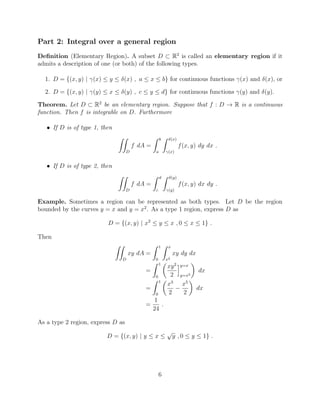
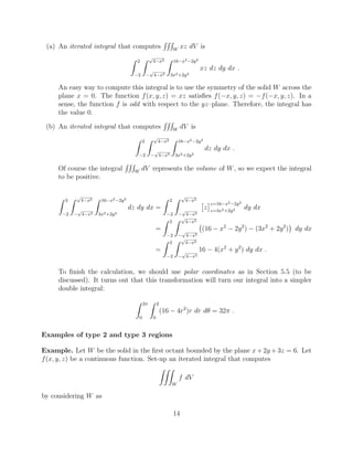
![Part 2: Integral over a general region
Definition (Elementary Region). A subset W ⇢ R3
is called an elementary region if it
admits a description of at least one of the following types.
1. Type 1 Regions [The most fundamental of regions]
(a) W = {(x, y, z) | '(x, y) z (x, y) , (x) y (x) , a x b} , or
(b) W = {(x, y, z) | '(x, y) z (x, y) , ↵(y) x (y) , c y d} .
Simply put, the region W is the region between the graphs of z = '(x, y) and z =
(x, y) over an elementary region in the xy–plane.
2. Type 2 Regions
(a) W = {(x, y, z) | ↵(y, z) x (y, z) , (z) y (z) , p z q} , or
(b) W = {(x, y, z) | ↵(y, z) x (y, z) , '(y) z (y) , c y d} .
Simply put, the region W is the region between the graphs of x = ↵(y, z) and x =
(y, z) over an elementary region in the yz–plane.
3. Type 3 Regions
(a) W = {(x, y, z) | (x, z) y (x, z) , ↵(z) x (z) , p z q} , or
(b) W = {(x, y, z) | (x, y) y (x, y) , '(x) z (x) , a x b} .
Simply put, the region W is the region between the graphs of y = (x, z) and y = (x, z)
over an elementary region in the xz–plane.
Theorem. Let W be an elementary region in R3
and let f be a function on W.
1. If W is a type 1 region, then
ZZZ
W
f dV =
Z b
a
Z (x)
(x)
Z (x,y)
'(x,y)
f(x, y, z) dz dy dx ,
or ZZZ
W
f dV =
Z d
c
Z (y)
↵(y)
Z (x,y)
'(x,y)
f(x, y, z) dz dx dy .
2. If W is a type 2 region, then
ZZZ
W
f dV =
Z q
p
Z (z)
(z)
Z (y,z)
↵(y,z)
f(x, y, z) dx dy dz ,
or ZZZ
W
f dV =
Z d
c
Z (y)
'(y)
Z (y,z)
↵(y,z)
f(x, y, z) dx dz dy .
11](https://image.slidesharecdn.com/notesuptoch7sec3-140410165830-phpapp01/85/Notes-up-to_ch7_sec3-11-320.jpg)
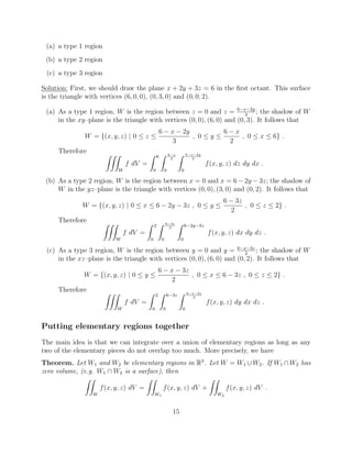
![Linear change of variables for integrals
Theorem (Linear change of variables). Suppose that T : R2
uv ! R2
xy is an invertible
linear transformation. Suppose that D⇤
⇢ R2
uv and D ⇢ R2
xy are elementary regions
such that T(D⇤
) = D. If f : D ! R is continuous, then
ZZ
D
f(x, y) dx dy =
ZZ
D⇤
f(x(u, v), y(u, v)) | det T| du dv .
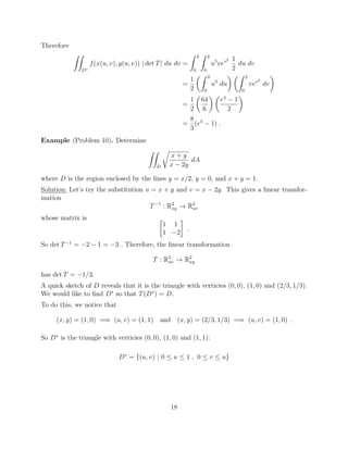
Example (Problem 9). Evaluate the integral
Z 2
0
Z (x/2)+1
x/2
x5
(2y x)e(2y x)2
dy dx
by making the substitution u = x and v = 2y x.
Solution:
The substitution u = x and v = 2y x gives a linear transformation
T 1
: R2
xy ! R2
uv
whose matrix is
1 0
1 2
.
So det T 1
= 2. Therefore, the linear transformation
T : R2
uv ! R2
xy
has det T = 1/2.
A quick sketch of the region D reveals that D is the parallelogram spanned by the vectors
(2, 1) and (0, 1). We would like to find D⇤
so that T(D⇤
) = D.
To do this, we notice that
(x, y) = (2, 1) =) (u, v) = (2, 0) and (x, y) = (0, 1) =) (u, v) = (0, 2) .
It follows that D⇤
is the parallelogram spanned by the vectors (2, 0) and (0, 2). Hence
D⇤
= {(u, v) | 0 u 2 , 0 v 2} = [0, 2] ⇥ [0, 2] .
17](https://image.slidesharecdn.com/notesuptoch7sec3-140410165830-phpapp01/85/Notes-up-to_ch7_sec3-17-320.jpg)
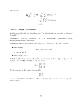
![Since T 1
is an a ne (linear + translation) transformation, it takes straight-lines to straight-
lines. It follows that D⇤
= T 1
(D) is a parallelogram with vertices T 1
(0, 0) = ( 3, 6),
T 1
(2, 1) = (2, 6), T 1
(3, 1) = (2, 1), and T 1
(1, 2) = ( 3, 1). Therefore
D⇤
= [ 3, 2] ⇥ [1, 6] .
Therefore
ZZ
D
(2x + y 3)2
(2y x + 6)2
dx dy =
ZZ
D⇤
u2
v2
·
1
5
du dv =
Z 2
3
Z 6
1
u2
5v2
dv du =
35
18
.
Example (Simple rescaling). Consider the linear transformation T : R2
uv ! R2
xy defined by
(x, y) = T(u, v) = (2u, 3v) .
It is easy to see that T transforms the unit square
[0, 1] ⇥ [0, 1] ⇢ R2
uv
into the rectangle
[0, 2] ⇥ [0, 3] ⇢ R2
xy .
Also, T transforms the unit disk
D⇤
= {(u, v) | u2
+ v2
1} ⇢ R2
uv
into the elliptical region
D = {(x, y) | (x/2)2
+ (y/3)2
1} ⇢ R2
xy .
The determinant of T is
det T = 6 .
This linear transformation allows us to compute
Area(D) =
ZZ
D
1 dx dy =
ZZ
D⇤
|det T| du dv = |det T|
✓ZZ
D⇤
1 du dv
◆
= 6·Area(D⇤
) = 6⇡ .
Review of polar coordinates (See section 1.7)
Polar coordinates are also called angular coordinates. These are the best coordinates for
describing geometric objects that possesses circular symmetry. The coordinates are (r, ✓);
here r represents the radial coordinate and ✓ represents the angular (or circular) coordinate.
Example (Disk). Consider the closed disk centered at the origin with radius 2:
D = {(x, y) | x2
+ y2
4} .
We can describe this region in polar coordinates as
D⇤
= {(r, ✓) | 0 r 2 , 0 ✓ 2⇡} .
21](https://image.slidesharecdn.com/notesuptoch7sec3-140410165830-phpapp01/85/Notes-up-to_ch7_sec3-21-320.jpg)

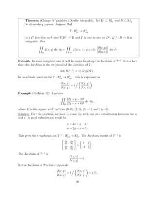
![Example (Polar coordinates with a twist). Consider the curve
4x2
+ y2
8x + 4y 8 = 0
in R2
. This curve is an ellipse:
4x2
+ y2
8x + 4y 8 = 0 =) 4(x2
2x) + (y2
+ 4y) = 8
=) 4(x2
2x + 1) + (y2
+ 4y + 4) = 8 + 4 + 4
=) 4(x 1)2
+ (y + 2)2
= 16
=)
✓
x 1
2
◆2
+
✓
y + 2
4
◆2
= 1 .
Suppose that we want to integrate a continuous function f(x, y) over the region D bounded
by this ellipse:
D =
(
(x, y)
✓
x 1
2
◆2
+
✓
y + 2
4
◆2
1
)
.
We could use an a ne (linear + translation) change of variables
u =
x 1
2
, v =
y + 2
4
and then change to polar coordinates, or we can do everything at once.
Consider the substitution
r cos ✓ =
x 1
2
, r sin ✓ =
y + 2
4
.
This substitution corresponds to the transformation
T : R2
r✓ ! R2
xy
defined by the equations
x = 2r cos ✓ + 1 , y = 4r sin ✓ 2 .
Just like in ordinary polar coordinates, we have D⇤
= [0, 1] ⇥ [0, 2⇡] ⇢ R2
r✓.
The Jacobian matrix for T is
DT =
" @x
@r
@x
@✓
@y
@r
@y
@✓
#
=
2 cos ✓ 2r sin ✓
4 sin ✓ 4r cos ✓
.
So the Jacobian determinant is
@(x, y)
@(r, ✓)
= det DT = 8r cos2
✓ + 8r sin2
✓ = 8r .
For instance, we can now directly compute the area of D :
Area(D) =
ZZ
D
1 dx dy =
ZZ
D⇤
8r dr d✓ =
Z 2⇡
0
Z 1
0
8r dr d✓ = 8⇡ .
25](https://image.slidesharecdn.com/notesuptoch7sec3-140410165830-phpapp01/85/Notes-up-to_ch7_sec3-25-320.jpg)
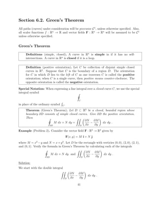
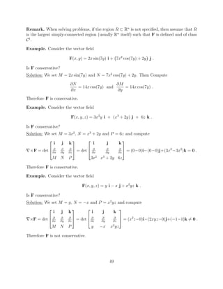
![Section 6.1. Scaler and vector line integrals
It will be useful for you to review parts of Chapter 3.
All paths (curves) under consideration will be piecewise C1
, unless otherwise specified. Also,
all scaler functions f : Rn
! R and vector fields F : Rn
! Rn
will be assumed to be
continuous unless otherwise specified.
The following is a useful way to parametrize a straight line connecting two points P and Q.
Straight-line parametrizations: A convenient way to get a parametrization of
a line segment in Rn
beginning at a point P and ending at a point Q is to use the
formula
x(t) = (1 t)P + tQ .
This gives a straight-line path
x : [0, 1] ! Rn
with x(0) = P and x(1) = Q.
Scaler line integrals
Let x : [a, b] ! Rn
be a path. Let f : Rn
! R be given. Then the scaler line integral of
f along x is
Z
x
f ds =
Z b
a
f(x(t)) ||x0
(t)|| dt .
Notice that ||x0
(t)|| is the speed. In particular, the length of the path is given by integrating
the speed:
length(x) =
Z
x
1 ds =
Z b
a
||x0
(t)|| dt .
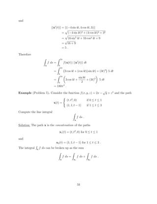
Example (Problem 4). Let f(x, y, z) = 3x + xy + z3
. Consider the parametrization
x(t) = (cos 4t, sin 4t, 3t)
for 0 t 2⇡. Compute
R
x
f ds.
Solution:
f(x(t)) = 3 cos 4t + (cos 4t)(sin 4t) + (3t)3
33](https://image.slidesharecdn.com/notesuptoch7sec3-140410165830-phpapp01/85/Notes-up-to_ch7_sec3-33-320.jpg)
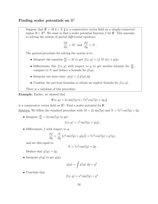
![We see that
Z
x1
f ds =
Z 1
0
f(x1(t)) ||x0
1(t)|| dt
=
Z 1
0
(2t t) ||(1, 2t, 0)|| dt
=
Z 1
0
t
p
1 + 4t2 dt
=
Z 5
1
p
u
8
du
⇥
substitute u = 1 + 4t2
=) du = 8t dt
⇤
=
p
125 1
12
.
Also
Z
x2
f ds =
Z 3
1
f(x2(t)) ||x0
2(t)|| dt
=
Z 3
1
(1 + (t 1)2
) ||(0, 0, 1)|| dt
=
Z 3
1
(1 + (t 1)2
) dt
=
14
3
.
Therefore,
Z
x
f ds =
p
125 1
12
+
14
3
.
Vector line integrals
This time, the integrand will be a vector field.
Let x : [a, b] ! Rn
be a path. Let F : Rn
! Rn
be a vector field. Then the vector line
integral of F along x is
Z
x
F · ds =
Z b
a
F(x(t)) · x0
(t) dt .
Example. Let F(x, y, z) = 3xi + y2
j + 6zk = (3, y2
, 6z). Consider the path x(t) = (t, 3, 5t2
)
defined for 0 t 1. Compute
R
x
F · ds .
Solution:
F(x(t)) = (3t, 9, 30t2
)
35](https://image.slidesharecdn.com/notesuptoch7sec3-140410165830-phpapp01/85/Notes-up-to_ch7_sec3-35-320.jpg)
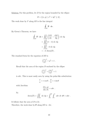
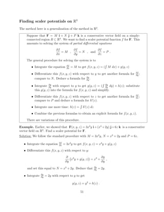
![and
x0
(t) = (1, 0, 10t) .
Therefore,
Z
x
F · ds =
Z b
a
F(x(t)) · x0
(t) dt
=
Z 1
0
(3t, 9, 30t2
) · (1, 0, 10t) dt
=
Z 1
0
3t + 300t3
dt
=
153
2
.
Di↵erential form
Suppose that we are given a vector field F : R2
! R2
defined by
F(x, y) = M(x, y)i + N(x, y)j
and a path x : [a, b] ! R2
. We can express the formula of the line integral
Z
x
F · ds
as Z
x
(M(x, y), N(x, y)) · (x0
(t), y0
(t)) dt =
Z
x
[M(x, y)x0
(t) + N(x, y)y0
(t)] dt .
If we multiply dt into the rest of integrand and use the di↵erentials
dx = x0
(t) dt , and dy = y0
(t) dt
we get the di↵erential form
Z
x
F · ds =
Z
x
M dx + N dy .
The same is true for a vector field on R3
F(x, y, z) = M(x, y, z)i + N(x, y, z)j + P(x, y, z)k
and a path
x : [a, b] ! R3
.
The vector line integral of F along x has the di↵erential form
Z
x
F · ds =
Z
x
M dx + N dy + P dz .
36](https://image.slidesharecdn.com/notesuptoch7sec3-140410165830-phpapp01/85/Notes-up-to_ch7_sec3-36-320.jpg)
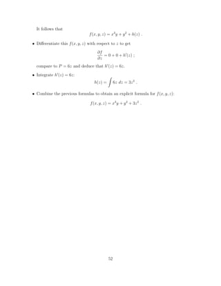
![Example. Consider the path
x : [0, 1] ! R3
defined by the formula x(t) = (t, t2
, t3
). Compute
Z
x
2x dx + z dy + y dz .
Solution: Compute the di↵erentials
dx = x0
(t) dt = 1 dt , dy = y0
(t) dt = 2t dt , dz = z0
(t) dt = 3t2
dt .
Then substitute
Z
x
2x dx + z dy + y dz =
Z 1
0
2t dt + (t3
)(2t dt) + t2
(3t2
dt) =
Z 1
0
(2t + 2t4
+ 3t4
) dt = 2 .
Example (Compare with problem 22). Calculate
Z
C
z dx x dy + 2y dz
where C is the curve obtained by intersecting the surfaces z = x2
and x2
+ y2
= 4 and
oriented counterclockwise around the z–axis (as seen from the positive z–axis).
Solution:
Since C is the intersection of two surfaces, we want a parametrization
x : [a, b] ! R3
, x(t) = (x(t), y(t), z(t))
which satisfies both equations
x2
+ y2
= 4 and z = x2
.
Start with the equation x2
+ y2
= 4 because the shadow of C in the xy–plane will be the
circle x2
+ y2
= 4. The standard (counterclockwise) parametrization of that circle in R2
is
(2 cos t, 2 sin t) , 0 t 2⇡ .
Since C also lies on the surface z = x2
, we just set z(t) = (x(t))2
= (2 cos t)2
= 4 cos2
t .
It follows that the parametrization for C should be
x : [0, 2⇡] ! R3
, x(t) = (2 cos t, 2 sin t, 4 cos2
t) .
The di↵erentials are
dx = 2 sin t dt , dy = 2 cos t dt , dz = 8 cos t sin t dt .
37](https://image.slidesharecdn.com/notesuptoch7sec3-140410165830-phpapp01/85/Notes-up-to_ch7_sec3-37-320.jpg)
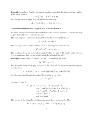
![Therefore,
Z
C
z dx x dy + 2y dz =
Z 2⇡
0
(4 cos2
t)( 2 sin t) dt (2 cos t)(2 cos t) dt + 2(2 sin t)( 8 cos t sin t) dt
=
Z 2⇡
0
( 8 cos2
sin t 4 cos2
t 32 sin2
t cos t) dt
= 4⇡ .
The e↵ect of reparametrization
Example. The image of each of the parametrizations
x : [0, 2⇡] ! R2
, x(t) = (cos t, sin t)
and
y : [0, ⇡] ! R2
, y(t) = (cos 2t, sin 2t)
is the unit circle {(x, y) | x2
+ y2
= 1}.
Definition. A reparametrization of a path
x : [a, b] ! Rn
is another path
y : [c, d] ! Rn
for which there exists a one-to-one and onto function u : [c, d] ! [a, b] with the
property y(t) = x(u(t)).
Furthermore, if u(c) = a, then y is an orientation-preserving reparametrization
of x; if u(c) = b, then y is an orientation-reversing reparametrization of x.
Two quick and easy way to see if the reparametrization preserves or reverses orientation is:
1. If you know u(t), then u0
(t) is negative if and only if y reverses orientation.
2. y reverses orientation if and only if the tangent (velocity) vectors for y and x point in
di↵erent directions at the same point on the image curve.
Example. In the previous example, we see that y is a reparametrization of x with
u : [0, ⇡] ! [0, 2⇡] , u(t) = 2t .
Notice that y preserves orientation.
38](https://image.slidesharecdn.com/notesuptoch7sec3-140410165830-phpapp01/85/Notes-up-to_ch7_sec3-38-320.jpg)
![Definition (Opposite path). Suppose that
x : [a, b] ! Rn
is a path. The opposite path
xopp : [a, b] ! Rn
is defined by
xopp(t) = x(a + b t) .
Example. The opposite path of
x : [0, 2⇡] ! R2
, x(t) = (cos t, sin t)
is
xopp : [0, 2⇡] ! R2
, x(t) = (cos(2⇡ t), sin(2⇡ t)) = (cos t, sin t).
The path x traces the unit circle in the counter-clockwise direction while the opposite path
xopp traces the unit circle in the clockwise direction.
Theorem (Reparametrization and scaler line integrals). Let
x : [a, b] ! Rn
be a path. Let f : Rn
! R. If
y : [c, d] ! Rn
is a reparametrization of x, then
Z
x
f ds =
Z
y
f ds .
Since scaler line integrals are not a↵ected by reparametrizations, we can define scaler line
integrals over curves without having to refer to parametrizations until we need them.
Example. Let be the upper half of the unit circle
= {(x, y) | x2
+ y2
= 1, y 0} .
We would like to integrate the function f(x, y) = y along . Consider the parametrization
x : [0, ⇡] ! R2
, x(t) = (cos t, sin t) .
So x0
(t) = ( sin t, cos t), and
Z
x
y ds =
Z ⇡
0
sin t
p
sin2
t + cos2 t dt =
Z ⇡
0
sin t dt = 2 .
39](https://image.slidesharecdn.com/notesuptoch7sec3-140410165830-phpapp01/85/Notes-up-to_ch7_sec3-39-320.jpg)
![Now consider another parametrization
y : [ 1, 1] ! R2
, y(t) = (t,
p
1 t2) .
So y0
(t) = (1, t/
p
1 t2), and
Z
y
y ds =
Z 1
1
p
1 t2
r
1 +
t2
1 t2
!
dt =
Z 1
1
dt = 2 .
Theorem (Reparametrization and vector line integrals). Let
x : [a, b] ! Rn
be a path. Let F : Rn
! Rn
be a vector field. Suppose that
y : [c, d] ! Rn
is a reparametrization of x.
1. If y preserves orientation, then
R
y
F · ds =
R
x
F · ds.
2. If y reverses orientation, then
R
y
F · ds =
R
x
F · ds.
Example. Let F : R2
! R2
be the vector field F(x, y) = xyi + y2
j. Consider the path
x : [0, 4] ! R2
, x(t) = (t, t2
) .
Then Z
x
F · ds =
Z 4
0
(t3
, t4
) · (1, 2t) dt =
Z 4
0
t3
+ 2t5
dt =
4288
3
.
Consider the reparametrization
y : [ 4, 0] ! R2
, y(t) = ( t, t2
) .
Notice that y reverses orientation. Then
Z
y
F · ds =
Z 0
4
( t3
, t4
) · ( 1, 2t) dt =
Z 0
4
t3
+ 2t5
dt =
4288
3
.
40](https://image.slidesharecdn.com/notesuptoch7sec3-140410165830-phpapp01/85/Notes-up-to_ch7_sec3-40-320.jpg)
![D is just the rectangle [0, 2] ⇥ [0, 1], so
ZZ
D
✓
@N
@x
@M
@y
◆
dx dy =
ZZ
D
(1 ( 1)) dx dy
=
Z 1
0
Z 2
0
2 dx dy
= 4 .
Now take care of the line integral
I
@D
M dx + N dy .
This is more labor-intensive:
The boundary @D consists of four line-segments 1, 2, 3, and 4 where
• 1 connects (0, 0) to (2, 0)
• 2 connects (2, 0) to (2, 1)
• 3 connects (2, 1) to (0, 1)
• 4 connects (0, 1) to (0, 0).
The simplest parametrizations for these segments (with the appropriate orientations) are the
following.
• 1 is given by x1 : [0, 2] ! R2
, x1(t) = (t, 0)
• 2 is given by x2 : [0, 1] ! R2
, x2(t) = (2, t)
• 3 is given by x3 : [0, 1] ! R2
, x3(t) = (1 t)2, 1
• 4 is given by x4 : [0, 1] ! R2
, x4(t) = (0, 1 t)
Then
I
@D
M dx + N dy =
4X
i=1
✓Z
xi
M dx + N dy
◆
= 4 .
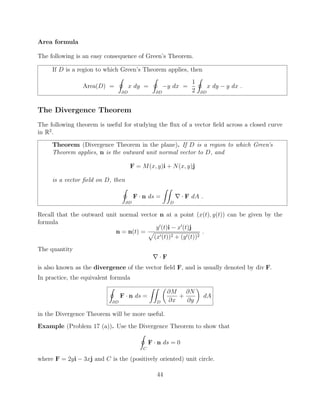
Example (Problem 8). Find the work done by the force field
F = (4y 3x)i + (x 4y)j
along the positively oriented ellipse
x2
+ 4y2
= 4 .
42](https://image.slidesharecdn.com/notesuptoch7sec3-140410165830-phpapp01/85/Notes-up-to_ch7_sec3-42-320.jpg)
![So the normal vector is
N = Ts ⇥ Tt =
✓
@f
@s
,
@f
@t
, 1
◆
.
For example, consider the graph of the function f(x, y) = x2
+ xey
on the domain D = R2
.
Give the graph of f(x, y) the standard parametrization
X(s, t) = (s, t, s2
+ set
) .
Then
N =
✓
@f
@s
,
@f
@t
, 1
◆
= (2s + et
), set
, 1 .
At the point (1, 0, 2) on the graph of f, the equation of the tangent plane is
N(1, 0)·(x 1, y, z 2) = 0 =) ( 3, 1, 1)·(x 1, y, z 2) = 0 =) 3(x 1) y+(z+2) = 0 .
This simplifies to
3x + y z = 1 .
Piecewise smooth parametrized surfaces
Definition (Piecewise parametrized surface). A piecewise parametrized sur-
face is the union of parametrized surfaces X : Di ! R3
, i = 1, . . . , m where
• Each Xi is of class C1
, except possibly along @Di.
• Each Si = X(Di) is smooth, except possibly at finitely many points.
Examples. The following are examples of piecewise smooth parametrized surfaces.
• The boundary of the solid cube [0, 1] ⇥ [0, 1] ⇥ [0, 1] ⇢ R3
. See Figure 7.12 in the
textbook.
• The boundary of nearly every solid that appears in section 5.4. In particular, see
Figures 5.47, 5.56, 5.63, 5.65 and 5.67 in the textbook.
Example. Consider the cylindrical solid
{(x, y, z) | x2
+ y2
1, 0 z 1} ⇢ R3
.
Let S denote the boundary of the solid. Then S consists of three smooth pieces S1, S2, S3:
• S1 = {(x, y, 0) | x2
+ y2
1} is the bottom of the cylinder.
57](https://image.slidesharecdn.com/notesuptoch7sec3-140410165830-phpapp01/85/Notes-up-to_ch7_sec3-57-320.jpg)
![• S2 = {(x, y, 1) | x2
+ y2
1} is the top of the cylinder.
• S3 = {(x, y, z) | x2
+ y2
= 1, 0 z 1} is the lateral portion of S.
See Figure 7.29 in the textbook. Notice that each Si is a smooth parametrized surface. So
when you need to calculate something over S, you can use parametrizations such as the
following.
• For S1, use X1(r, ✓) = (r cos ✓, r sin ✓, 0) , (r, ✓) 2 [0, 1] ⇥ [0, 2⇡].
• For S2, use X2(r, ✓) = (r cos ✓, r sin ✓, 1) , (r, ✓) 2 [0, 1] ⇥ [0, 2⇡].
• For S3, use X3(✓, z) = (cos ✓, sin ✓, z) , (✓, z) 2 [0, 2⇡] ⇥ [0, 1].
Area of a parametrized surface
Let X : D ! R3
be a parametrized surface. The surface area of S = X(D) is
defined to be ZZ
D
||Ts ⇥ Tt|| ds dt =
ZZ
D
||N(s, t)|| ds dt .
Example. Let S be the portion of the paraboloid z = 25 x2
y2
that lies over the xy–plane.
Find the area of S.
Solution 1: We can realize S as the graph of f(x, y) = 25 x2
y2
on the domain D ⇢ R2
where D is the shadow of S in the xy–plane. It is easy to see that D is the disk
D = {(x, y) | x2
+ y2
25} .
So consider the standard parametrization
X(s, t) = (s, t, 25 s2
t2
) .
Then
Ts = (1, 0, 2s) and Tt = (0, 1, 2t) .
So
||Ts ⇥ Tt|| = ||(2s, 2t, 1)|| =
p
(2s)2 + (2t)2 + 1 .
The area of S is
ZZ
D
||Ts ⇥ Tt|| ds dt =
ZZ
D
p
(2s)2 + (2t)2 + 1 ds dt .
To evaluate this integral, we should use polar coordinates for D. Make the substitutions
s = r cos ✓ , t = r sin ✓ ( 0 r 5 , 0 ✓ 2⇡ )
58](https://image.slidesharecdn.com/notesuptoch7sec3-140410165830-phpapp01/85/Notes-up-to_ch7_sec3-58-320.jpg)
![to get
ZZ
D
p
(2s)2 + (2t)2 + 1 ds dt =
Z 2⇡
0
Z 5
0
p
(2r cos ✓)2 + (2r sin ✓)2 + 1 r dr d✓
=
Z 2⇡
0
Z 5
0
p
4r2 + 1 r dr d✓
=
⇡
6
⇣
101
p
101 1
⌘
.
Solution 2: Consider the following (cylindrical) parametrization of S:
X : [0, 5] ⇥ [0, 2⇡] ! R3
, X(r, ✓) = (r cos ✓, r sin ✓, 25 r2
) .
This time, D is just the rectangle [0, 5] ⇥ [0, 2⇡]. Then
Tr = (cos ✓, sin ✓, 2r) and T✓ = ( r sin ✓, r cos ✓, 0) .
So
Tr ⇥ T✓ = (2r2
cos ✓, 2r2
sin ✓, r cos2
✓ + r sin2
✓) = (2r2
cos ✓, 2r2
sin ✓, r) .
The area of S is
ZZ
D
||Tr ⇥ T✓|| dr d✓ =
Z 2⇡
0
Z 5
0
p
4r4 cos2 ✓ + 4r4 sin2
✓ + r2 dr d✓
=
Z 2⇡
0
Z 5
0
p
4r4 + r2 dr d✓
=
Z 2⇡
0
Z 5
0
r
p
4r2 + 1 dr d✓
=
⇡
6
⇣
101
p
101 1
⌘
.
Remark. If S is a piecewise smooth parametrized surface where the smooth pieces S1, . . . , Sm
of S meet along curves, then calculate the area of S in a piecewise way:
Area(S) = Area(S1) + · · · + Area(Sm) .
59](https://image.slidesharecdn.com/notesuptoch7sec3-140410165830-phpapp01/85/Notes-up-to_ch7_sec3-59-320.jpg)
![Section 7.2. Surface integrals
Scaler surface integrals
Definition. Let X : D ! R3
be a smooth parametrized surface, where D ⇢ R2
is
a bounded region. Let f be a continuous scaler function on S = X(D). The scaler
surface integral of f along X is
ZZ
X
f dS =
ZZ
D
f X(s, t) ||Ts ⇥ Tt|| ds dt =
ZZ
D
f X(s, t) ||N(s, t)|| ds dt .
The definition extends to piecewise smooth parametrized surfaces.
Example. Let D = [0, 1] ⇥ [0, 2] and consider the parametrized surface
X(s, t) = (s, s + t, t) .
Compute
RR
X
x2
+ y2
+ z2
dS.
Solution: The coordinate tangent vectors are
Ts = (1, 1, 0) and Tt = (0, 1, 1) ,
so the normal vector Ts ⇥ Tt is
Ts ⇥ Tt = (1, 1, 1) ; so ||Ts ⇥ Tt|| =
p
3 .
Therefore
ZZ
X
x2
+ y2
+ z2
dS =
Z 2
0
Z 1
0
(s2
+ (s + t)2
+ t2
)
p
3 ds dt =
26
p
3
.
Vector surface integrals
Definition. Let X : D ! R3
be a smooth parametrized surface, where D ⇢ R2
is
a bounded region. Let F(x, y, z) be a continuous vector field on S = X(D). Then
the vector surface integral of F along X is
ZZ
X
F · dS =
ZZ
D
F X(s, t) · N(s, t) ds dt .
This integral is also known as a flux integral because it computes the flux of a
vector field F in R3
though the surface S.
60](https://image.slidesharecdn.com/notesuptoch7sec3-140410165830-phpapp01/85/Notes-up-to_ch7_sec3-60-320.jpg)
![Example. Consider the vector field F(x, y, z) = 2x i+y j z k on the parametrized surface
X : [0, 1] ⇥ [0, 2] ! R3
, X(s, t) = (s + t, t, st) .
Compute ZZ
X
F · dS .
Solution: The coordinate tangent vectors are
Ts = (1, 0, t) and Tt = (1, 1, s) ,
so the normal vector is
N(s, t) = Ts ⇥ Tt = ( t, t s, 1) .
Therefore
ZZ
X
F · dS =
Z 2
0
Z 1
0
2(s + t), t, st · t, t s, 1 ds dt
=
Z 2
0
Z 1
0
2t(s + t) + t(t s) st ds dt
=
Z 2
0
Z 1
0
t2
4st ds dt
=
20
3
.
The e↵ect of reparametrization
The situation is similar to the one for line integrals, the scaler integrals do not depend on
reparametrization, and the same is true for vector integrals (up to ± sign).
Definition. A reparametrization of a surface
X : D1 ! R3
is another parametrization
Y : D2 ! R3
for which there exists a di↵erentiable coordinate transformation H : D2 ! D1 that
is one-to-one and onto, and Y(s, t) = X(H(s, t)).
61](https://image.slidesharecdn.com/notesuptoch7sec3-140410165830-phpapp01/85/Notes-up-to_ch7_sec3-61-320.jpg)
![• A suitable parametrization for S3 is
X3 : [0, 2⇡] ⇥ [0, 1] ! R3
, X3(✓, z) = (cos ✓, sin ✓, z) .
Notice that
@X3
@✓
= ( sin ✓, cos ✓, 0) and
@X3
@z
= (0, 0, 1) =) N3 =
@X3
@✓
⇥
@X3
@z
= (cos ✓, sin ✓, 0) .
The outward normal vector is N3.
Now consider the vector field
F(x, y, z) = x i 2y j + (x2
+ z) k
on R3
. Then the flux of F through S is
ZZ
S
F · dS =
ZZ
S1
F · dS +
ZZ
S2
F · dS +
ZZ
S3
F · dS
=
ZZ
D
(s, 2t, s2
) · (0, 0, 1) ds dt +
ZZ
D
(s, 2t, s2
) · (0, 0, 1) ds dt
+
Z 2⇡
0
Z 1
0
(cos ✓, 2 sin ✓, cos2
✓ + z) · (cos ✓, sin ✓, 0) dz d✓
=
ZZ
D
s2
ds dt +
ZZ
D
s2
ds dt +
Z 2⇡
0
Z 1
0
(cos2
✓ 2 sin2
✓) dz d✓
= 0 ⇡/2
= ⇡/2 .
65](https://image.slidesharecdn.com/notesuptoch7sec3-140410165830-phpapp01/85/Notes-up-to_ch7_sec3-65-320.jpg)
![The boundary of W consists of two pieces
S1 = {(x, y, 0) | x2
+ y2
9} and S2 = {(x, y, z) | z = 9 x2
y2
, z 0}
With S1 and S2 properly oriented, we can compute
RR
@W
F · dS as the sum
ZZ
@W
F · dS =
ZZ
S1
F · dS +
ZZ
S2
F · dS .
Let D dentote the closed disk {(s, t) | s2
+ t2
9} ⇢ R2
.
For S1, we can use the parametrization
X1 : D ! R3
, X1(s, t) = (s, t, 0)
as long as we use the downward pointing normal vector
N1 = (0, 0, 1) .
Thus ZZ
S1
F · dS =
ZZ
D
(2s, 5t, 0) · (0, 0, 1) ds dt =
ZZ
D
0 ds dt = 0 .
For S2, we can use the parametrization
X2 : D ! R3
, X2(s, t) = (s, t, 9 s2
t2
)
with the upward pointing normal vector
N2 = (2s, 2t, 1) .
This yields
ZZ
S2
F · dS =
ZZ
S2
2s, 5t, 3(9 s2
t2
) · (2s, 2t, 1) ds dt
=
ZZ
D
(s2
+ 7t2
+ 27) ds dt
Then change to polar coordinates
s = r cos ✓ , t = r sin ✓
for (r, ✓) 2 [0, 3] ⇥ [0, 2⇡].
70](https://image.slidesharecdn.com/notesuptoch7sec3-140410165830-phpapp01/85/Notes-up-to_ch7_sec3-70-320.jpg)
![The integral is now
ZZ
S2
F · dS =
ZZ
D
(s2
+ 7t2
+ 27) ds dt
=
Z 2⇡
0
Z 3
0
(r2
cos2
✓ + 7r2
sin2
✓ + 27) r dr d✓
=
Z 2⇡
0
Z 3
0
(r2
+ 6r2
sin2
✓ + 27) r dr d✓
= 405⇡ .
Therefore ZZ
@W
F · dS = 0 + 405⇡ = 405⇡ .
Example. Let S be the boundary of the cube C = [ 1, 1]3
; orient S with normal vectors
that point into C. Consider the vector field
F(x, y, z) =
✓
x
⇢3
,
y
⇢3
,
z
⇢3
◆
where ⇢ = ⇢(x, y, z) =
p
x2 + y2 + z2. Use the Divergence Theorem to compute the surface
integral ZZ
S
F · dS .
Solution:
The denominator ⇢3
in the components of F is problematic. It makes F is not defined at the
origin, so we can’t just set
RR
S
F · dS equal to
RRR
C
r · F dV .
The good news is that the Divergence Theorem allows us to integrate F over large spheres
instead of over S:
First, we compute the divergence of F: Use the quotient rule to compute the necessary
partial derivatives:
@
@x
✓
x
⇢3
◆
=
⇢2
3x2
⇢5
@
@y
✓
y
⇢3
◆
=
⇢2
3y2
⇢5
@
@z
✓
z
⇢3
◆
=
⇢2
3z2
⇢5
.
71](https://image.slidesharecdn.com/notesuptoch7sec3-140410165830-phpapp01/85/Notes-up-to_ch7_sec3-71-320.jpg)

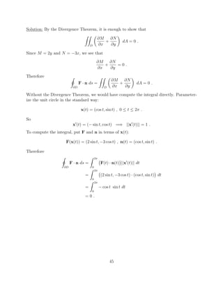
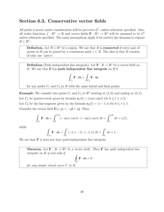
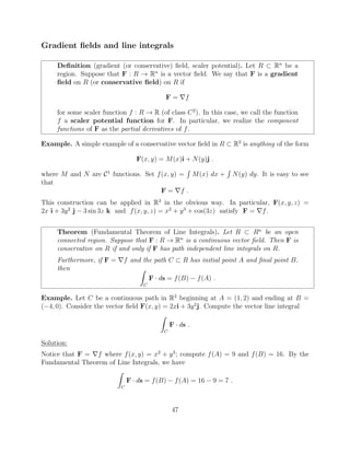
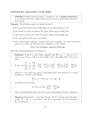
This document provides an overview of key concepts in multivariable calculus covered in MAT 10B at Williams College in Fall 2011, including: 1) Definitions and computations of double integrals, including over rectangles and more general regions, and Fubini's theorem on changing the order of integration. 2) Triple integrals as a generalization of double integrals to functions of three variables over boxes in R3. 3) Techniques for changing the order of integration in iterated integrals when one order may be more convenient than another.


