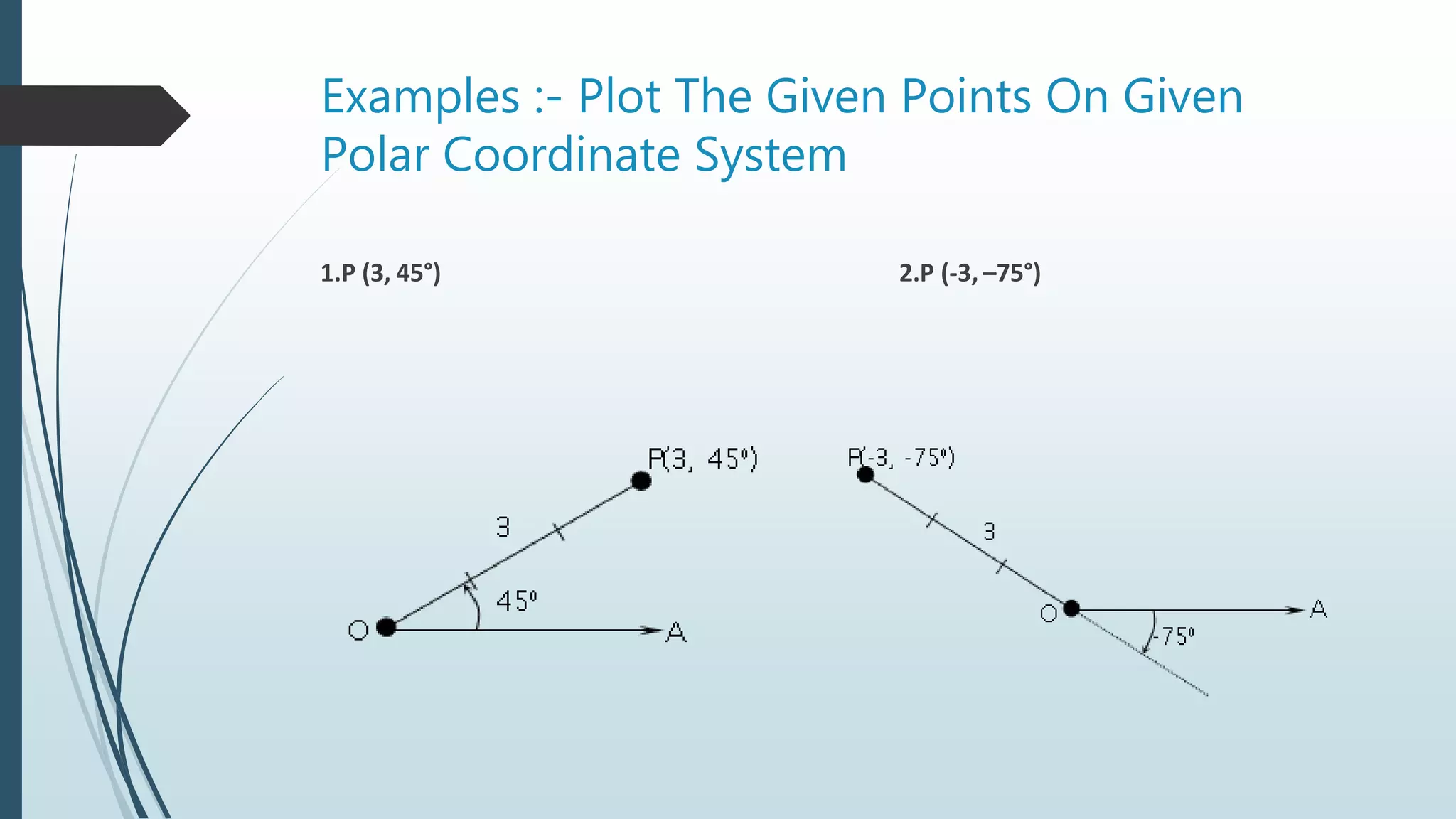
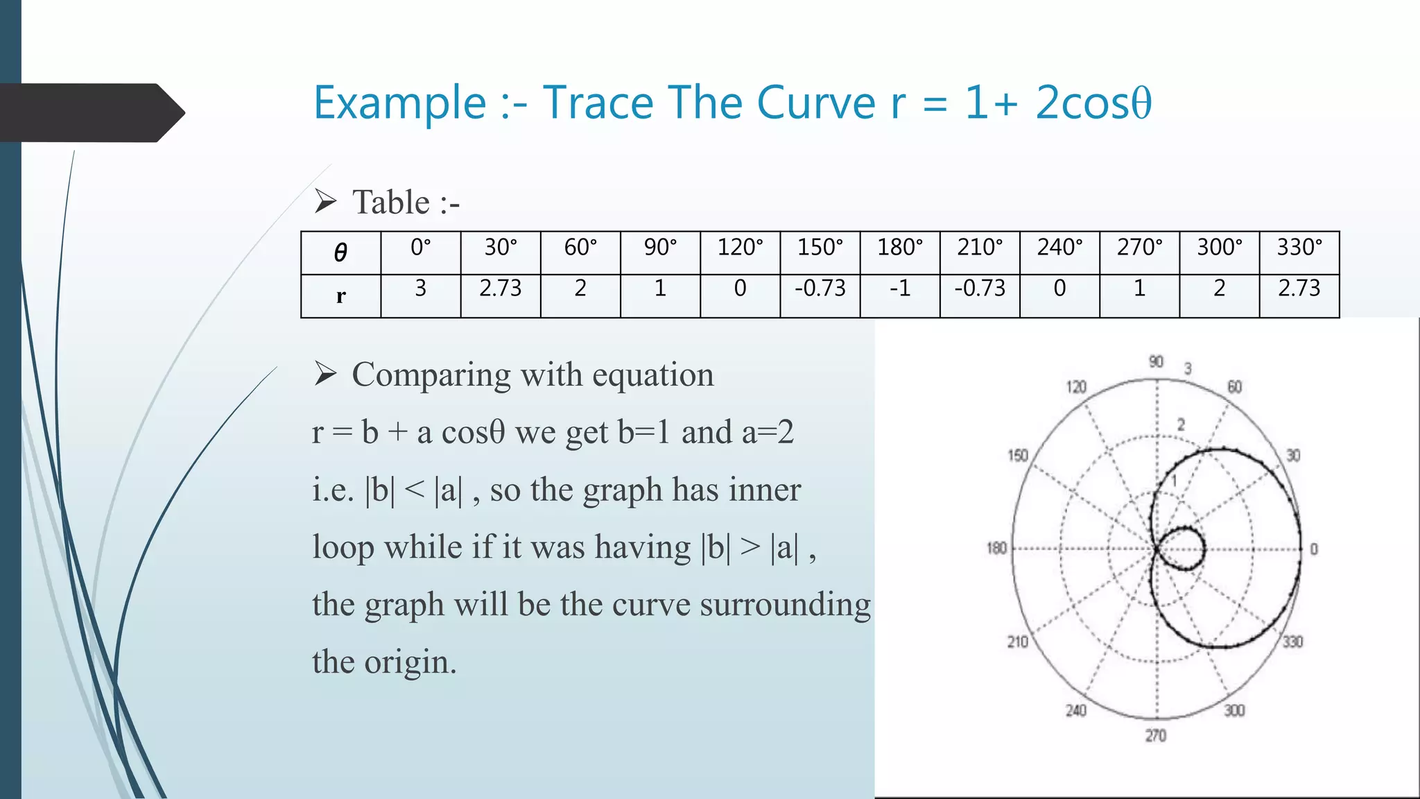
The document discusses polar coordinates, defining them as a system based on distances from a fixed point and directions from a fixed line. It covers the relationship between polar and rectangular coordinates, examples of plotting points, and the graphs of polar equations including special types like rose curves and limacons. The submission is for a group project at Sarvajanik College of Engineering and Technology, guided by Prof. Dixa P. Kevadiya.

1. Sarvajanik College Of Engineering
And Technology
Calculus(2110014)
Computer Engineering Eve. (COE)
Date Of Submission :- 13/11/2017

2. Group Members And Topic
 55 – Ms. Shakshi Mehta
 56 – Mr. Priyank Bardoliya
 57 – Mr. Keyur Vadodariya
 58 – Ms. Rishika Jain
 59 – Mr. Pathik Thakor
Topic:- Polar Curves
 Guided By :- Prof. Dixa P. Kevadiya

3. The Polar Co-ordinate System
 The Polar Coordinates System is a coordinate system in which the
coordinates of a point in a plane are its distances from a fixed point
and its direction from a fixed line. The fixed point is called the
origin or the pole and the fixed line is called the polar axis. The
coordinates given in this way are called Polar Coordinates.
Where:
O - Origin or Pole
OA - Polar Axis
r - Radius Vector
θ - Vectorial Angle
P(r, θ) – Polar Coordinate

4. Sign Convection
 For Vectorial Angle (θ):
• Positive (+) – If it is measured counterclockwise from the polar axis.
• Negative (-) – If it is measured clock wise from the polar axis.
 For Radius Vector (r):
• Positive (+) – If it is measures from the pole along the terminal side
of Vectorial angle (θ).
• Negative (-) – If it is measured along the terminal side extended
through the pole.

5. Examples :- Plot The Given Points On Given
Polar Coordinate System
1.P (3, 45°) 2.P (-3, –75°)

6. Relation Between Rectangular And Polar
Coordinates
 The transformation formulas that express the relationship between
rectangular coordinates and polar coordinates of a point are as
follows:

7. Example :- Find the rectangular coordinates of
the points defined by the polar coordinates
(6,150°).

8. Graph Of Polar Equation
Eight-Leaf Rose
 The graph of an equation r = f(θ) in
polar coordinates is the set of all points
(r, θ) whose coordinates satisfy the
equation.
 Special Types Of Polar Curves :- Three-Leaf Rose
1.Rose Curve
r = a sin(nθ) or r = a cos(nθ), if n is odd,
There are n leaves; if n is even there are 2n
leaves.

9. 2.Spirals
Spiral Of Archimedes; r = aθ Logarithmic Spiral; r = eaθ
3.Limacon
r = b + asin(θ) or r = b + acos(θ), if a = b, the Limacon is called a Cardiod.

10. Example :- Trace The Curve r = 1+ 2cosθ
 Table :-
 Comparing with equation
r = b + a cosθ we get b=1 and a=2
i.e. |b| < |a| , so the graph has inner
loop while if it was having |b| > |a| ,
the graph will be the curve surrounding
the origin.
θ 0° 30° 60° 90° 120° 150° 180° 210° 240° 270° 300° 330°
r 3 2.73 2 1 0 -0.73 -1 -0.73 0 1 2 2.73