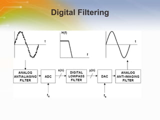
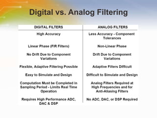
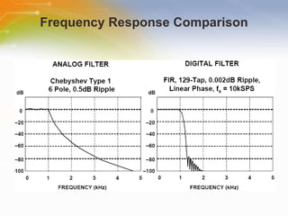
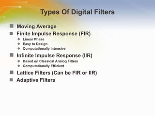
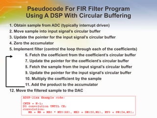
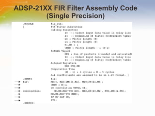
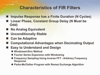
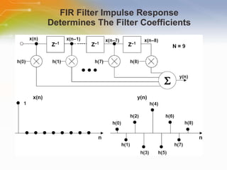
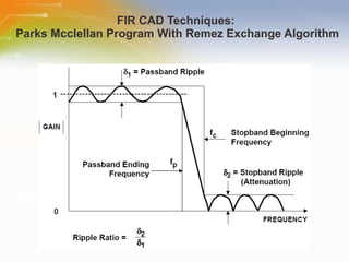
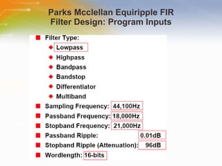
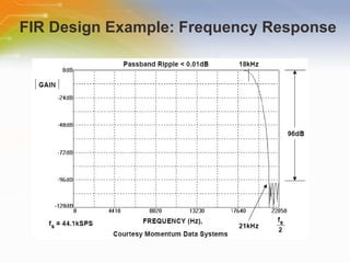
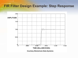
DIGITAL FILTERS Source: ANALOG DEVICES  Part1:Finite Impulse Response (FIR) Filters
Introduction Purpose This module introduce the  technology of Finite Impulse Response (FIR) Filters. Outline Introduce the technology of Digital Filters. Introduce the technology of Finite Impulse Response (FIR) Filters. Contents 32 pages Duration 20 Minutes
Digital Filtering
Digital vs. Analog Filtering
Frequency Response Comparison
Processing Requirements Signal Bandwidth = fa Sampling Frequency fs > 2fa Sampling Period = 1 / fs Filter Computational Time + Overhead < Sampling Period Depends on Number of Taps Speed of DSP Multiplication-Accumulates (MACs) Efficiency of DSP Circular Buffering Zero Overhead Looping
Types Of Digital Filters Moving   Average Finite   Impulse   Response   (FIR) Linear   Phase Easy   to   Design Computationally   Intensive Infinite   Impulse   Response   (IIR) Based   on   Classical   Analog   Filters Computationally   Efficient Lattice   Filters   (Can   be   FIR   or   IIR) Adaptive   Filters
4-point Moving Average Filter
Calculating Output Of 4-point Moving Average Filter
4-tap Moving Average Filter Step Response
Moving Average Filter Response To Noise Superimposed On Step Input
Moving Average Filter Frequency Response
N-tap Finite Impulse Response (FIR) Filter
Simplified Filter Notations
Calculating Outputs Of 4-tap FIR Filter  Using A Circular Buffer
Pseudocode For FIR Filter Program Using A DSP With Circular Buffering 1. Obtain sample from ADC (typically interrupt driven) 2. Move sample into input signal’s circular buffer 3. Update the pointer for the input signal’s circular buffer 4. Zero the accumulator 5. Implement filter (control the loop through each of the coefficients) 6. Fetch the coefficient from the coefficient’s circular buffer 7. Update the pointer for the coefficient’s circular buffer 8. Fetch the sample from the input signal’s circular buffer 9. Update the pointer for the input signal’s circular buffer 10. Multiply the coefficient by the sample 11. Add the product to the accumulator 12. Move the filtered sample to the DAC
ADSP-21XX FIR Filter Assembly Code (Single Precision)
Characteristics of FIR Filters Impulse Response has a Finite Duration (N Cycles) Linear Phase, Constant Group Delay (N Must be Odd) No Analog Equivalent Unconditionally Stable Can be Adaptive Computational Advantages when Decimating Output Easy to Understand and Design Windowed-Sinc Method Fourier Series Expansion with Windowing Frequency Sampling Using Inverse FFT - Arbitrary Frequency Response Parks-McClellan Program with Remez Exchange Algorithm
FIR Filter Impulse Response Determines The Filter Coefficients
Duality Of Time And Frequency
FIR Filter Design Using The Windowed-sinc Method
FIR Filter Design  Using Fourier Series Method With Windowing Specify   H(f) Expand   H(f)   in   a   Fourier   series:   The   Fourier   series   coefficients   are   the   coefficients   of   the   FIR   filter,   h(m),   and   its   Impulse   Response Truncate   the   Impulse   Response   to   N   points   (taps) Apply   a   suitable   Window   function   to   h(m)   to   smooth   the   effects   of   truncation Lacks   precise   control   of   cutoff   frequency;   Highly   dependent   on   Window   function
Frequency Sampling Method for FIR Filters With Arbitrary Frequency Response Specify H(k) as a Finite Number of Spectral Points Spread Uniformly Between 0 and 0.5fs (512 Usually Sufficient) Specify Phase Points (Can Make Equal to Zero) Convert Rectangular Form (Real + Imaginary)  Take the Complex Inverse FFT of H(k) Array to Obtain the Impulse Response Truncate the Impulse Response to N Points Apply a suitable Window function to h(m) to smooth the effects of Truncation Test Filter Design and Modify if Necessary CAD Design Techniques More Suitable for Lowpass, Highpass, Bandpass, or Bandstop Filters
FIR CAD Techniques:  Parks Mcclellan Program With Remez Exchange Algorithm
Parks Mcclellan Equiripple FIR Filter Design: Program Inputs
FIR Filter Program Outputs
FIR Design Example: Frequency Response
FIR Filter Design Example: Step Response
FIR Design Example: Impulse Response (Filter Coefficients)
Design Example Using ADSP-2189M: Processor Time for 69-TAP FIR Filter Sampling   Frequency   fs   =   44.1kSPS Sampling   Interval   =   1   /   fs   =   22.7μs Number   of   Filter   Taps,   N   =   69 Number   of   Required   Instructions   =   N   +   5   =   74 Processing   Time   /   Instruction   =   13.3ns   (75MIPS)   (ADSP-2189M) Total   Processing   Time   =   74×13.3ns   =   984ns Total   Processing   Time   <   Sampling   Interval   with   22.7μs   –   0.984μs   =   21.7μs   for   Other   Operations Increase   Sampling   Frequency   to   1MHz Use   Slower   DSP   (3.3MIPS) Add   More   Filter   Taps   (Up   to   N   =   1700)
Designing Highpass Filters using Lowpass Filter Impulse Response Spectral   Inversion   Technique: Design   Lowpass   Filter   (Linear   Phase,   N   odd) Change   the   Sign   of   Each   Coefficient   in   the   Impulse   Response,   h(m) Add   1   to   the   Coefficient   at   the   Center   of   Symmetry Spectral   Reversal   Technique: Design   Lowpass   Filter Change   the   Sign   of   Every   Other   Coefficient   in   the   Impulse   Response,   h(m) This   Reverses   the   Frequency   Domain   left-for-right:   0   becomes   0.5,   and   0.5   becomes   0;   i.e.,   if   the   cutoff   frequency   of   the   lowpass   filter   is   0.2,   the   cutoff   of   the   resulting   highpass   filter   is   0.3
Bandpass and Bandstop Filters Designed from Lowpass and Highpass Filters
Additional Resource For ordering the ADSP-21xx, please click the part list or Call our sales hotline For additional inquires contact our technical service hotline For more product information go to http://www.analog.com/en/embedded-processing-dsp/adsp-21xx/processors/index.html Newark Farnell

Digital Filters Part 1

  • 1.
    DIGITAL FILTERS Source:ANALOG DEVICES Part1:Finite Impulse Response (FIR) Filters
  • 2.
    Introduction Purpose Thismodule introduce the technology of Finite Impulse Response (FIR) Filters. Outline Introduce the technology of Digital Filters. Introduce the technology of Finite Impulse Response (FIR) Filters. Contents 32 pages Duration 20 Minutes
  • 3.
  • 4.
  • 5.
  • 6.
    Processing Requirements SignalBandwidth = fa Sampling Frequency fs > 2fa Sampling Period = 1 / fs Filter Computational Time + Overhead < Sampling Period Depends on Number of Taps Speed of DSP Multiplication-Accumulates (MACs) Efficiency of DSP Circular Buffering Zero Overhead Looping
  • 7.
    Types Of DigitalFilters Moving Average Finite Impulse Response (FIR) Linear Phase Easy to Design Computationally Intensive Infinite Impulse Response (IIR) Based on Classical Analog Filters Computationally Efficient Lattice Filters (Can be FIR or IIR) Adaptive Filters
  • 8.
  • 9.
    Calculating Output Of4-point Moving Average Filter
  • 10.
    4-tap Moving AverageFilter Step Response
  • 11.
    Moving Average FilterResponse To Noise Superimposed On Step Input
  • 12.
    Moving Average FilterFrequency Response
  • 13.
    N-tap Finite ImpulseResponse (FIR) Filter
  • 14.
  • 15.
    Calculating Outputs Of4-tap FIR Filter Using A Circular Buffer
  • 16.
    Pseudocode For FIRFilter Program Using A DSP With Circular Buffering 1. Obtain sample from ADC (typically interrupt driven) 2. Move sample into input signal’s circular buffer 3. Update the pointer for the input signal’s circular buffer 4. Zero the accumulator 5. Implement filter (control the loop through each of the coefficients) 6. Fetch the coefficient from the coefficient’s circular buffer 7. Update the pointer for the coefficient’s circular buffer 8. Fetch the sample from the input signal’s circular buffer 9. Update the pointer for the input signal’s circular buffer 10. Multiply the coefficient by the sample 11. Add the product to the accumulator 12. Move the filtered sample to the DAC
  • 17.
    ADSP-21XX FIR FilterAssembly Code (Single Precision)
  • 18.
    Characteristics of FIRFilters Impulse Response has a Finite Duration (N Cycles) Linear Phase, Constant Group Delay (N Must be Odd) No Analog Equivalent Unconditionally Stable Can be Adaptive Computational Advantages when Decimating Output Easy to Understand and Design Windowed-Sinc Method Fourier Series Expansion with Windowing Frequency Sampling Using Inverse FFT - Arbitrary Frequency Response Parks-McClellan Program with Remez Exchange Algorithm
  • 19.
    FIR Filter ImpulseResponse Determines The Filter Coefficients
  • 20.
    Duality Of TimeAnd Frequency
  • 21.
    FIR Filter DesignUsing The Windowed-sinc Method
  • 22.
    FIR Filter Design Using Fourier Series Method With Windowing Specify H(f) Expand H(f) in a Fourier series: The Fourier series coefficients are the coefficients of the FIR filter, h(m), and its Impulse Response Truncate the Impulse Response to N points (taps) Apply a suitable Window function to h(m) to smooth the effects of truncation Lacks precise control of cutoff frequency; Highly dependent on Window function
  • 23.
    Frequency Sampling Methodfor FIR Filters With Arbitrary Frequency Response Specify H(k) as a Finite Number of Spectral Points Spread Uniformly Between 0 and 0.5fs (512 Usually Sufficient) Specify Phase Points (Can Make Equal to Zero) Convert Rectangular Form (Real + Imaginary) Take the Complex Inverse FFT of H(k) Array to Obtain the Impulse Response Truncate the Impulse Response to N Points Apply a suitable Window function to h(m) to smooth the effects of Truncation Test Filter Design and Modify if Necessary CAD Design Techniques More Suitable for Lowpass, Highpass, Bandpass, or Bandstop Filters
  • 24.
    FIR CAD Techniques: Parks Mcclellan Program With Remez Exchange Algorithm
  • 25.
    Parks Mcclellan EquirippleFIR Filter Design: Program Inputs
  • 26.
  • 27.
    FIR Design Example:Frequency Response
  • 28.
    FIR Filter DesignExample: Step Response
  • 29.
    FIR Design Example:Impulse Response (Filter Coefficients)
  • 30.
    Design Example UsingADSP-2189M: Processor Time for 69-TAP FIR Filter Sampling Frequency fs = 44.1kSPS Sampling Interval = 1 / fs = 22.7μs Number of Filter Taps, N = 69 Number of Required Instructions = N + 5 = 74 Processing Time / Instruction = 13.3ns (75MIPS) (ADSP-2189M) Total Processing Time = 74×13.3ns = 984ns Total Processing Time < Sampling Interval with 22.7μs – 0.984μs = 21.7μs for Other Operations Increase Sampling Frequency to 1MHz Use Slower DSP (3.3MIPS) Add More Filter Taps (Up to N = 1700)
  • 31.
    Designing Highpass Filtersusing Lowpass Filter Impulse Response Spectral Inversion Technique: Design Lowpass Filter (Linear Phase, N odd) Change the Sign of Each Coefficient in the Impulse Response, h(m) Add 1 to the Coefficient at the Center of Symmetry Spectral Reversal Technique: Design Lowpass Filter Change the Sign of Every Other Coefficient in the Impulse Response, h(m) This Reverses the Frequency Domain left-for-right: 0 becomes 0.5, and 0.5 becomes 0; i.e., if the cutoff frequency of the lowpass filter is 0.2, the cutoff of the resulting highpass filter is 0.3
  • 32.
    Bandpass and BandstopFilters Designed from Lowpass and Highpass Filters
  • 33.
    Additional Resource Forordering the ADSP-21xx, please click the part list or Call our sales hotline For additional inquires contact our technical service hotline For more product information go to http://www.analog.com/en/embedded-processing-dsp/adsp-21xx/processors/index.html Newark Farnell