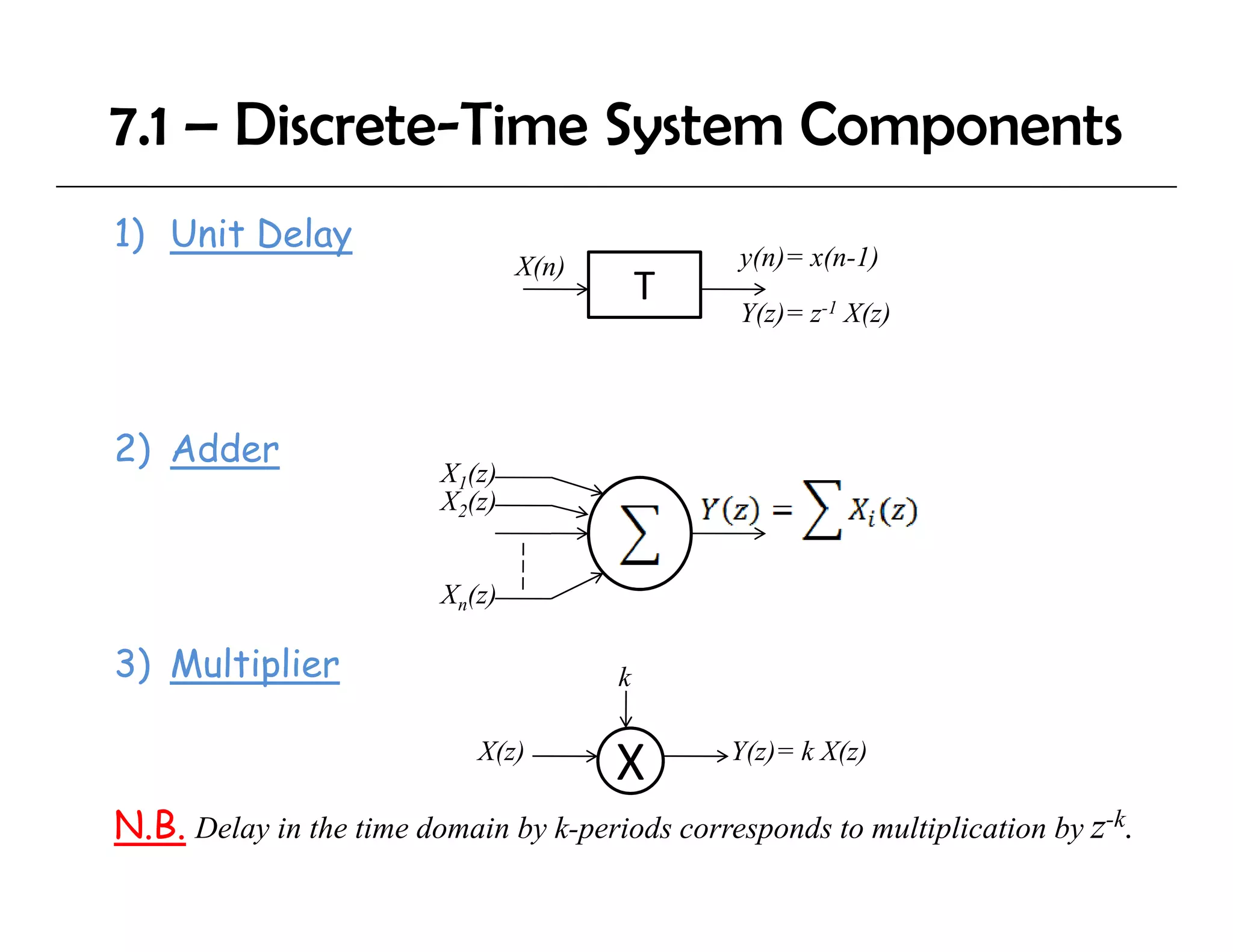
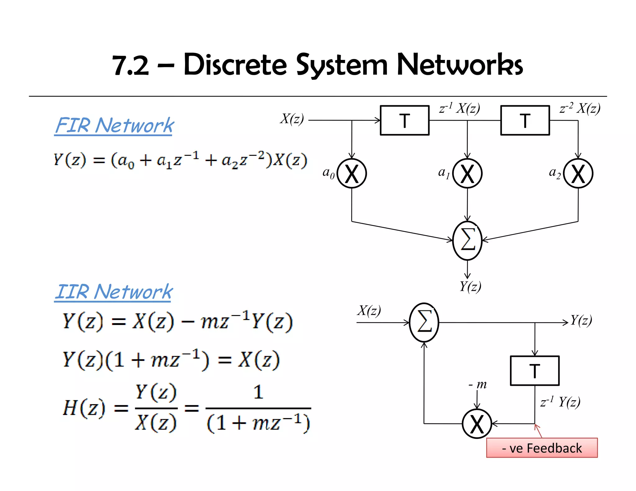
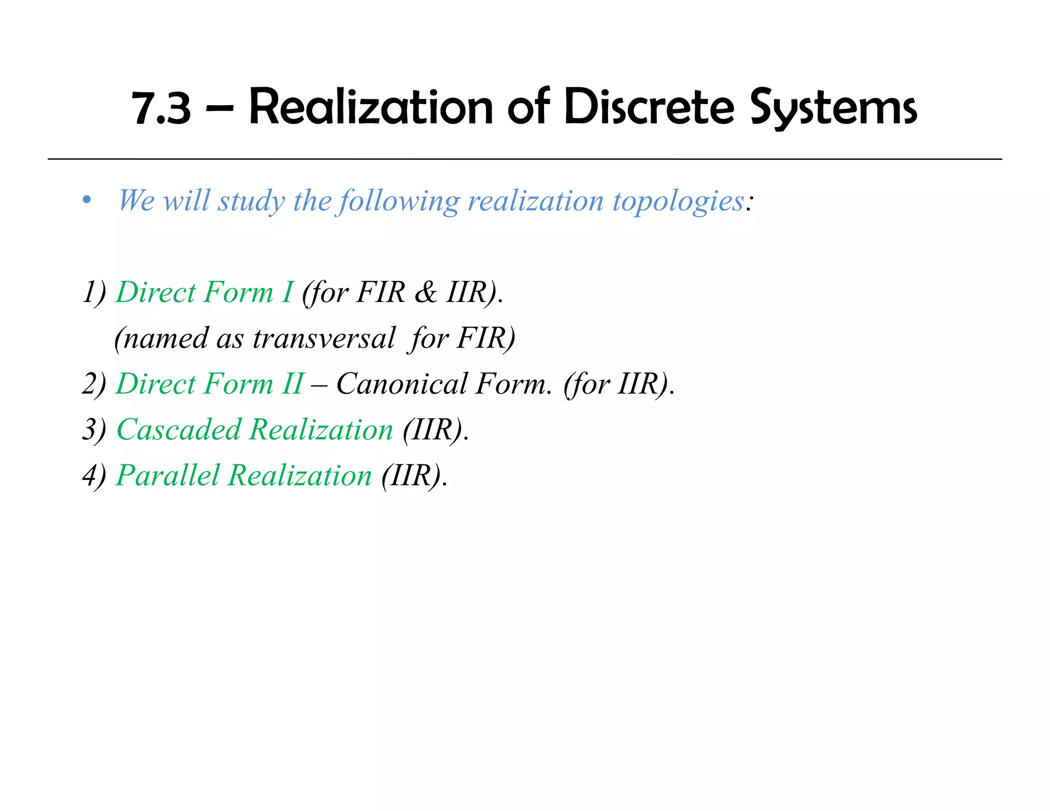
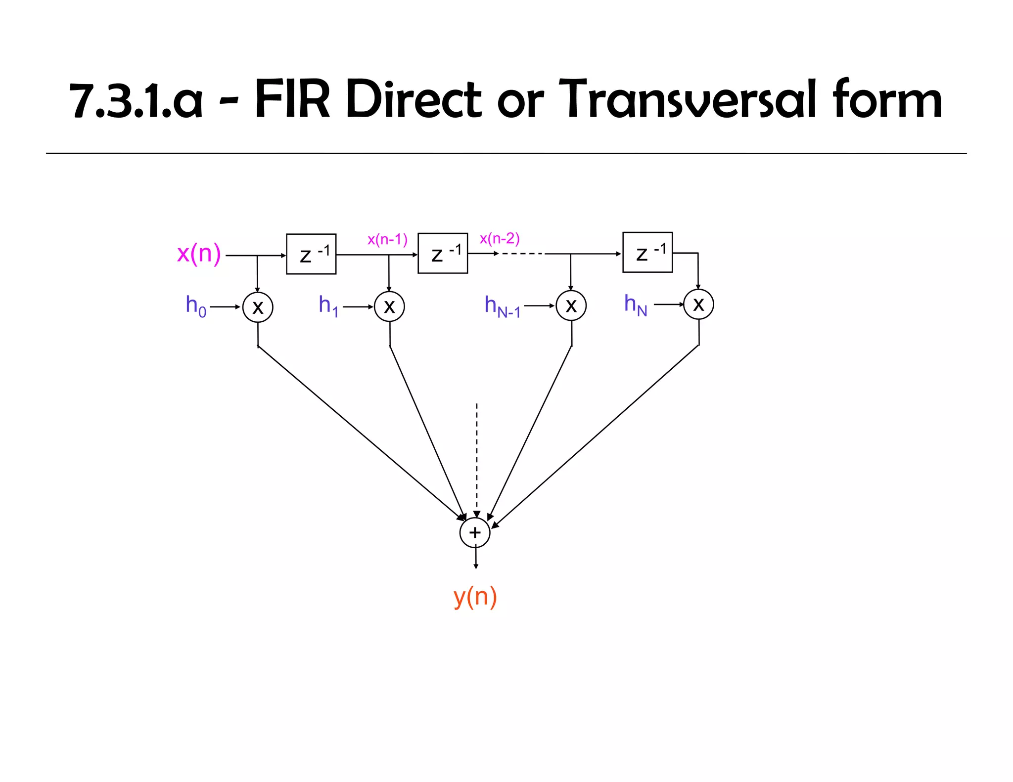
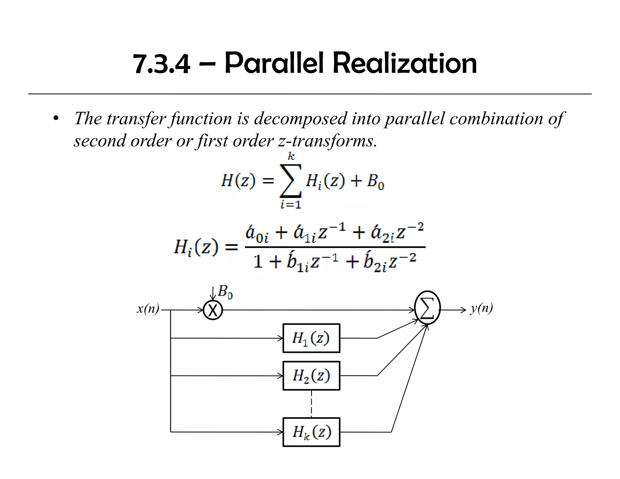
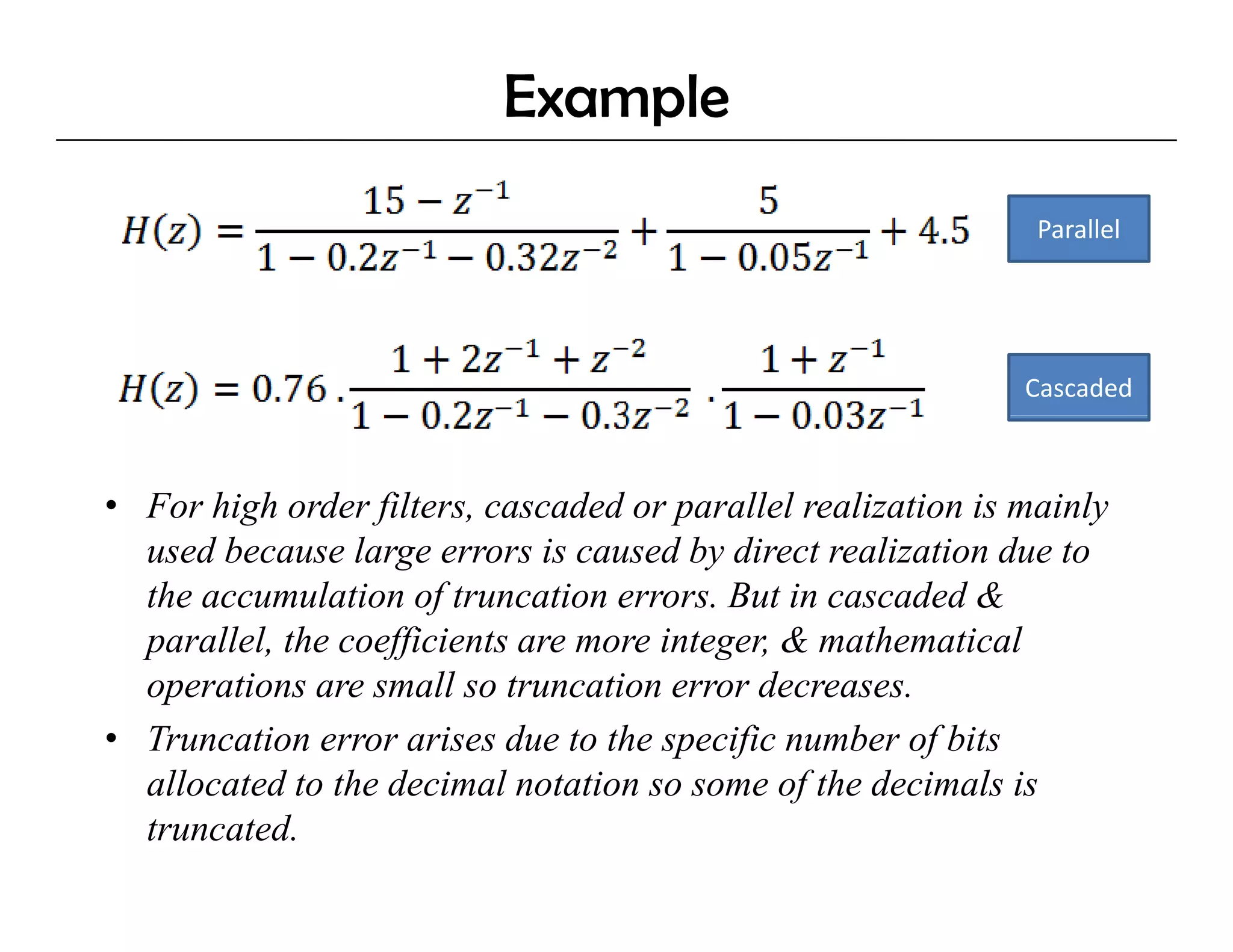
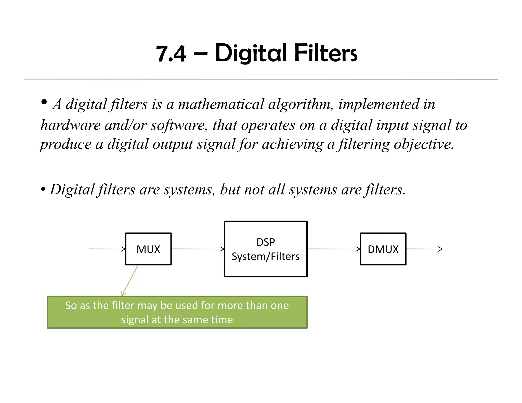
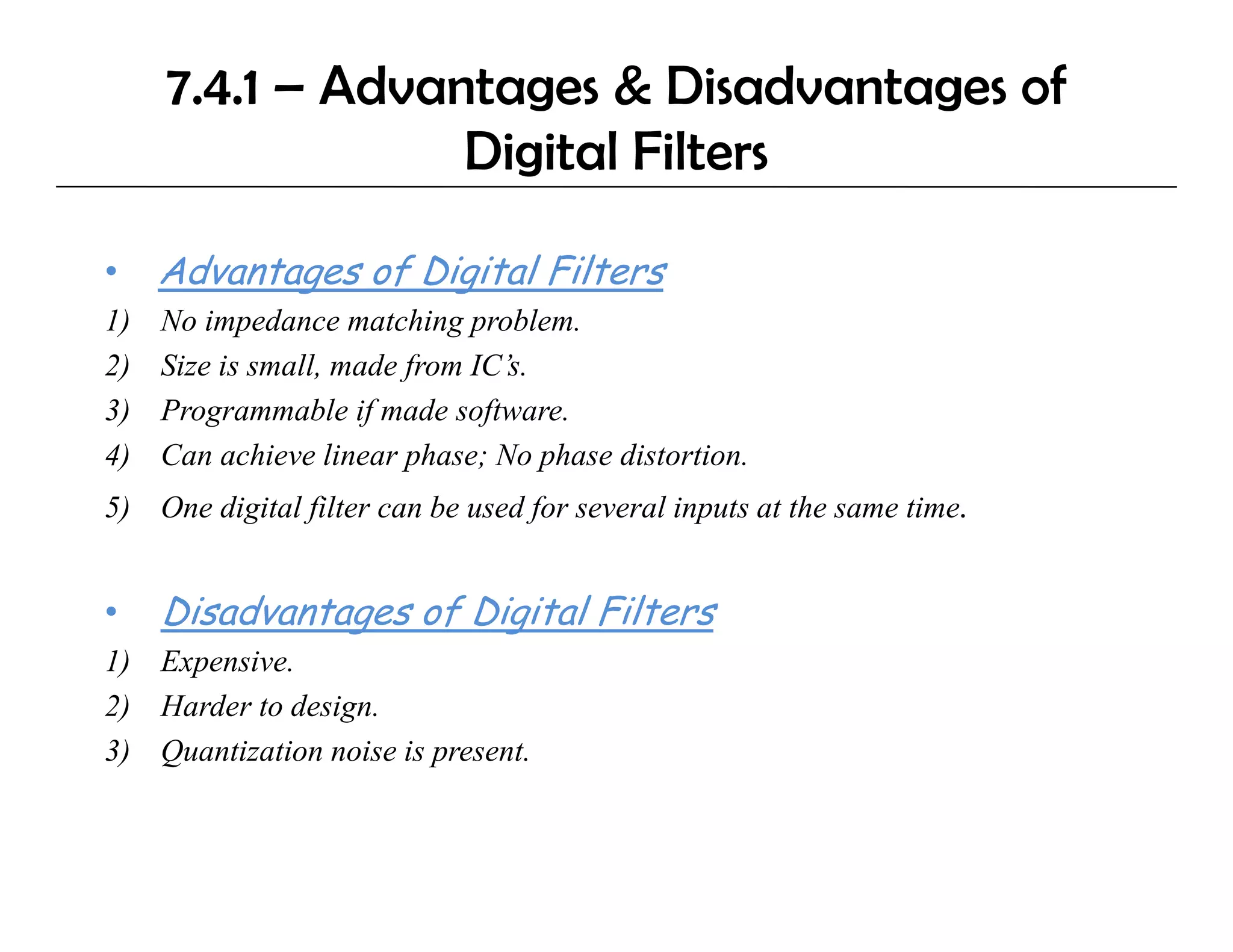
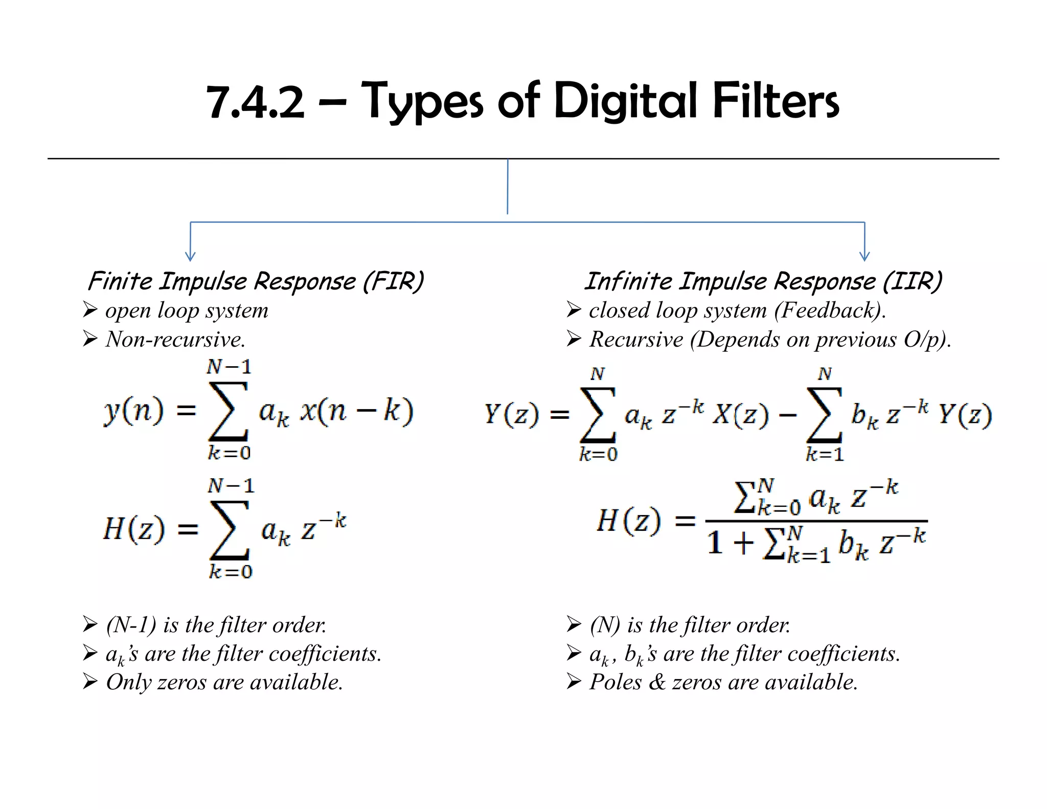
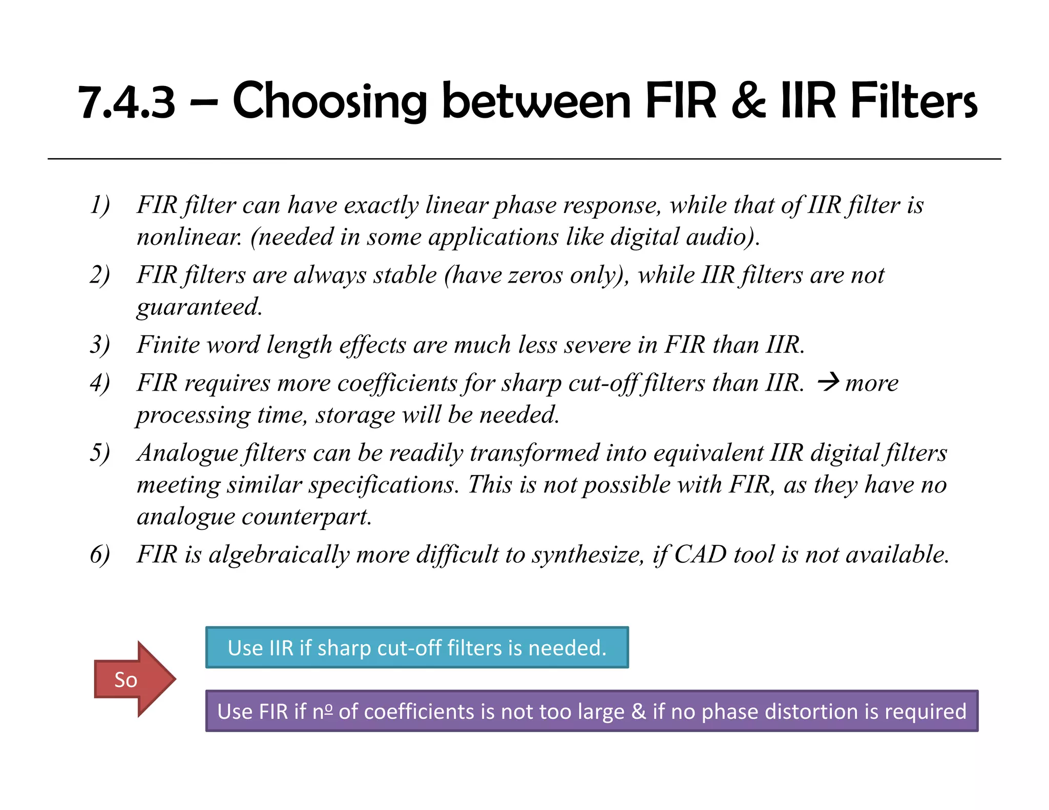
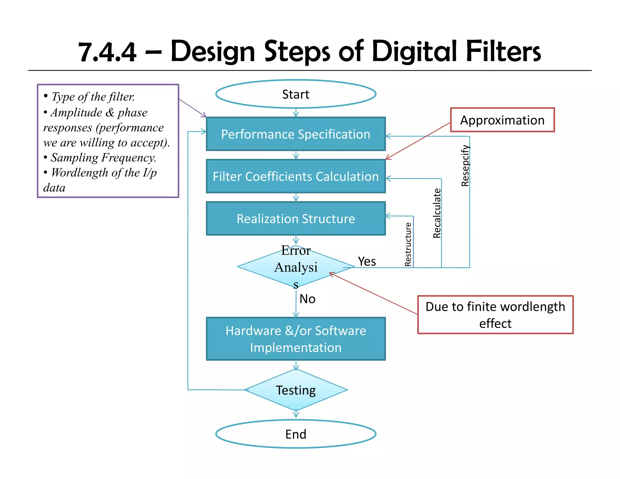
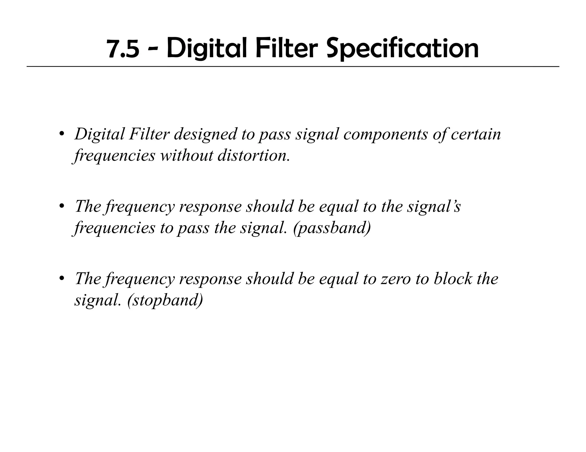
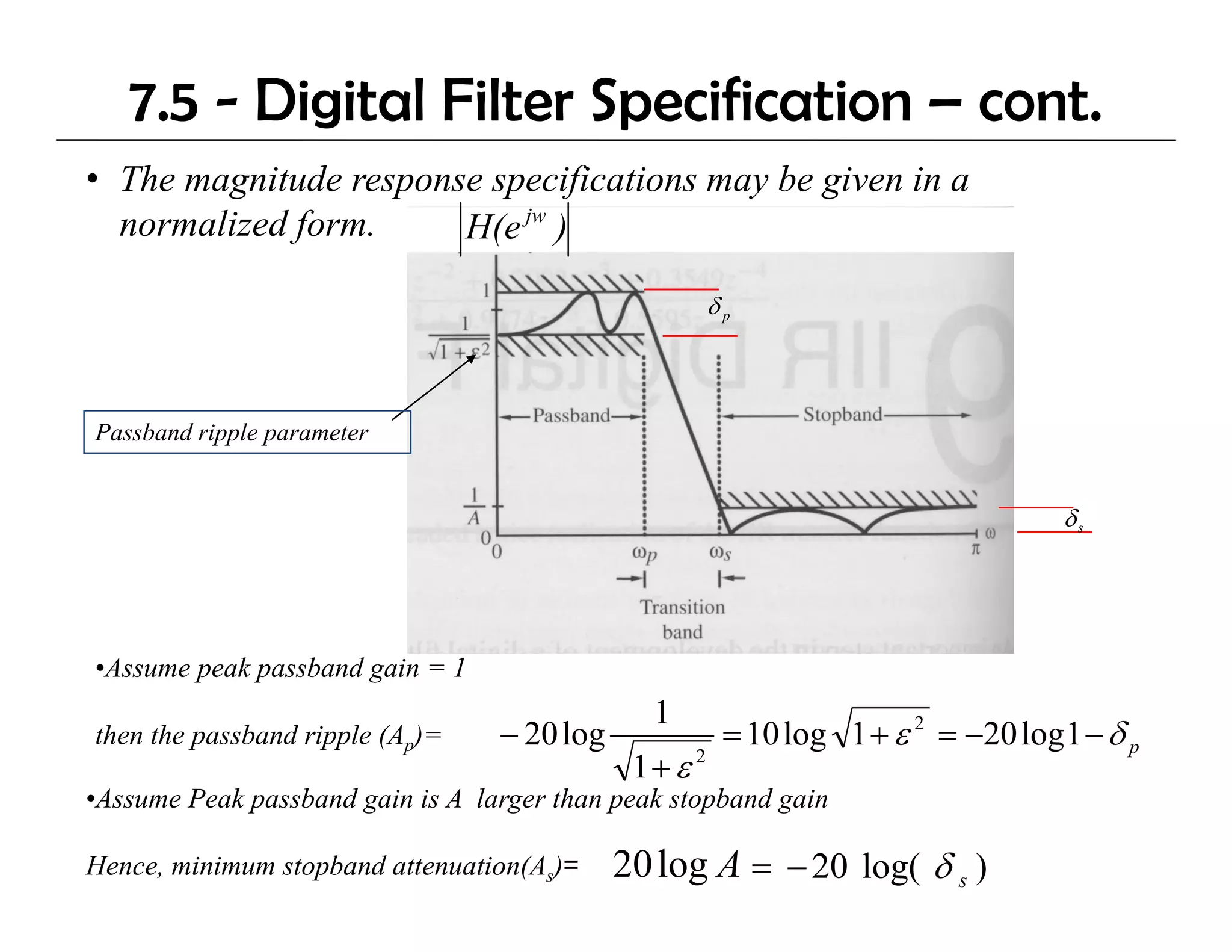
This document provides an overview of discrete-time systems and digital signal processing. It discusses discrete-time system components like unit delays and adders. It also covers discrete system networks including FIR and IIR networks. Various realizations of discrete systems are presented, including direct form I and II, cascaded, and parallel realizations. Digital filters are defined and the advantages and disadvantages as well as types (FIR and IIR) are discussed. Design steps and specifications for digital filters are also outlined.

1. EC533: Digital Signal Processing
5 l l
Lecture 7
Realization of Discrete-Time
Systems

2. 7.1 – Discrete-Time System Components
1) Unit Delay
X(n) y(n)= x(n-1)
T
Y(z)= z-1 X(z)
2) Adder
X1(z)
X2(z)
Xn(z)
3) M lti li
Multiplier k
X(z) Y(z)= k X(z)
X
N.B. Delay in the time domain by k-periods corresponds to multiplication by z-k.

3. 7.2 – Discrete System Networks
z-1 X(z) z-2 X(z)
FIR Network X(z) T T
a0
X a1
X a2
X
IIR Network Y(z)
X(z)
Y(z)
-m
T
z-1 Y( )
Y(z)
X
‐ ve Feedback

4. Example
Find the transfer function for the following IIR Network
a0
X(z)
X Y(z)
- b1
T a1
X X
- b2 T
X
1
2
From 1 & 2

5. 7.3 – Realization of Discrete Systems
• We will study the following realization topologies:
1) Direct Form I (for FIR & IIR).
(
(named as transversal for FIR)
f )
2) Direct Form II – Canonical Form. (for IIR).
3) Cascaded Realization (IIR).
4) Parallel Realization (IIR).

6. 7.3.1.a - FIR Direct or Transversal form
x(n 1)
x(n-1) x(n 2)
x(n-2)
x(n)
( ) z -1 z -1 z -1
1
h0 x h1 x hN-1 x hN x
+
y(n)

7. 7.3.1.b - IIR Direct Form I
Feedforward
Feedback
M
D′( z ) = ∑ bi z −i
i =1
x(n) y(n)

8. 7.3.1.b - Direct Form I – cont.
a0
x(n) X y(n)
T a1 - b1 T
X X
T a2 - b2 T
X X
T a3 - b3 T
X X
a0
x(n) X y(n)
T a1 - b1 T
X X
T a2 - b2 T
X X
T a3 - b3 T
X X

9. 7.3.2 – IIR Direct Form II (Canonical Form)
a0
x(n) y(n)
X
- b1 T T a1
X X
- b2 T T a2
X X
- b3 T T a3
X X
a0
x(n) y(n)
X
- b1 T a1
X X
- b2 T a2
No of Delays= Order of the
y
X X System.
- b3 T a3
Less than the previous method
X X

10. 7.3.3 – Cascaded Realization
• The transfer function is decomposed into cascaded combination of
second order or first order z-transforms.
z transforms.
where is either a 2nd or a 1st order section.
2nd order
d
1st order
x(n) y(n)

11. 7.3.4 – Parallel Realization
• The transfer function is decomposed into parallel combination of
second order or first order z-transforms.
f f
x(n) X y(n)

12. Example
Parallel
Cascaded
• For high order filters, cascaded or parallel realization is mainly
used because large errors is caused by direct realization due to
the accumulation of truncation errors. But in cascaded &
p
parallel, the coefficients are more integer, & mathematical
, ff g ,
operations are small so truncation error decreases.
• Truncation error arises due to the specific number of bits
allocated to the decimal notation so some of the decimals is
ll t d t th d i l t ti f th d i l i
truncated.

13. 7.4 – Digital Filters
• A digital filters is a mathematical algorithm, implemented in
hardware and/or software, that operates on a digital input signal to
software
produce a digital output signal for achieving a filtering objective.
• Digital filters are systems, but not all systems are filters.
DSP
MUX DMUX
System/Filters
So as the filter may be used for more than one
signal at the same time

14. 7.4.1 – Advantages & Disadvantages of
Digital Filters
g
• Advantages of Digital Filters
1) No impedance matching problem.
2) Size is small, made from IC’s.
3) Programmable if made software.
software
4) Can achieve linear phase; No phase distortion.
5) One digital filter can be used for several inputs at the same time.
• Disadvantages of Digital Filters
1) E
Expensive.
i
2) Harder to design.
3) Quantization noise is present.

15. 7.4.2 – Types of Digital Filters
Finite Impulse Response (FIR) Infinite Impulse Response (IIR)
open loop system closed loop system (Feedback).
Non-recursive. Recursive (Depends on previous O/p).
(N-1) is the filter order. (N) is the filter order.
ak’s are the filter coefficients.
s ak , bk’s are the filter coefficients.
s
Only zeros are available. Poles & zeros are available.

16. 7.4.3 – Choosing between FIR & IIR Filters
1) FIR filter can have exactly linear phase response, while that of IIR filter is
nonlinear. (needed in some applications like digital audio).
2) FIR filters are always stable (have zeros only), while IIR filters are not
guaranteed.
3) Finite word length effects are much less severe in FIR than IIR.
) g ff
4) FIR requires more coefficients for sharp cut-off filters than IIR. more
processing time, storage will be needed.
5) Analogue filters can be readily transformed into equivalent IIR digital filters
meeting similar specifications. This is not possible with FIR, as they have no
analogue counterpart.
6) FIR is algebraically more difficult to synthesize, if CAD tool is not available.
synthesize available
Use IIR if sharp cut‐off filters is needed.
So
Use FIR if no of coefficients is not too large & if no phase distortion is required

17. 7.4.4 – Design Steps of Digital Filters
• Type of the filter. Start
• Amplitude & phase
responses (performance
Approximation
Performance Specification
we are willing to accept).
g p)
Resepcify
y
• Sampling Frequency.
• Wordlength of the I/p Filter Coefficients Calculation
data
ulate
Recalcu
Realization Structure
Restructure
Error
Analysi Yes
s
No
Due to finite wordlength
effect
Hardware &/or Software
Hardware &/or Software
Implementation
Testing
End

18. 7.5 - Digital Filter Specification
• Digital Filter designed to pass signal components of certain
g g p g p f
frequencies without distortion.
• The frequency response should be equal to the signal’s
frequencies to pass the signal. (passband)
• The frequency response should be equal to zero to block the
signal. (stopband)

19. 7.5 - Digital Filter Specification – cont.
• The main four Filter Types:

20. 7.5 - Digital Filter Specification – cont.
• The magnitude response specifications are given some
acceptable tolerances.
H(e jw )

21. 7.5 - Digital Filter Specification – cont.
• Transition band is specified between the passband and the
stopband to permit the magnitude to drop off smoothly.
b d h d d ff hl
• In Passband
1 − δ p ≤ H ( e jω ) ≤ 1 + δ p , for ω ≤ ω p
• In Stopband
jω
H (e ) ≤ δ s , for ω s ≤ ω ≤ π
• Where δp and δs are peak ripple values, ωp are
p
passband edge f q
g frequency and ωs are stopband edge
y p g
frequency

22. 7.5 - Digital Filter Specification – cont.
• Digital f
g filter specification are often given in terms of loss
p f f g f
function,
A(ω) = -20 log10 |H(ejω)|
• Loss specification of a digital filter
– Peak passband ripple, Ap = 20 log10 (1 + δp) dB
– Mi i
Minimum stopband attenuation, As = -20 l 10 (δs) dB
t b d tt ti 20 log

23. 7.5 - Digital Filter Specification – cont.
• The magnitude response specifications may be given in a
normalized form. H(e jw )
δp
Passband ripple parameter
δs
•Assume peak passband gain = 1
1
then the passband ripple (Ap)= − 20 log = 10 log 1 + ε 2 = −20 log 1 − δ p
1+ ε 2
•Assume Peak passband gain is A larger than peak stopband gain
Hence, minimum stopband attenuation(As)= 20 log A = − 20 log( δ s )