Adaptive filter
Ahmed Shamel
10/13/2016
“Adaptive filter Theory “
By
Simon Haykin
” Adaptive filter “
By
B.Farhang boroujeny
” Adaptive Linear & Nonlinear Filters “
By
(Frank) XiangYang Gao
10/13/2016
References:
10/13/2016
Overview
Before we start we must understand some concept :
 The term filter is a “black box” that takes an input signal ,processes it, and
then returns an output signal that in some way modifies the input. For
example, if the input signal is noisy, then one would want a filter that
removes noise, but otherwise leaves the signal unchanged.
 we may use a filter to perform three basic information-processing tasks:
1. Filtering, which means the extraction of information about a quantity of
interest at time t by using data measured up to and including time t.
10/13/2016
2. Smoothing, which differs from filtering in that information about the
quantity of interest need not be available at time t , This means that in
the case of smoothing there is a delay in producing the result of
interest.
3. Prediction, which is the forecasting side of information processing. The
aim here is to derive information about what the quantity of interest will
be like at some time t + T in the future, for some z > 0, by using data
measured up to and including time t.
10/13/2016
Filter
linear Non linear
 We may classify filters into linear and nonlinear.
A filter is said to be linear if the 1) filtered 2) smoothed 3) predicted
quantity at the output of the device is a linear function of the observations
applied w the filter input. Otherwise, the filter is nonlinear.
Fixed versus Adaptive Filter Design
10/13/2016
W0 , W1 , W2 ,…….. Wn-1Fixed
Determine the values of the coefficients of the digital filter that meet the
desired specifications and the values are not changed once they are
implemented
The coefficient values are not fixed. They are adjusted to optimize some
measure of the filter performance using incoming input data and error.
W0(n) , W1(n) , W2(N),….Wn-1(N)Adaptive
 The figure shows a filter emphasizing the way it is used in typical
problems.
The filter is used to reshape certain input signals in such a way that
its output is a good estimate of the given desired signal.
10/13/2016
Introduction To adaptive filter
Filter (A.F)Input signal Output signal
Desired
signal
Error signal+
Introduction To adaptive filter
10/13/2016
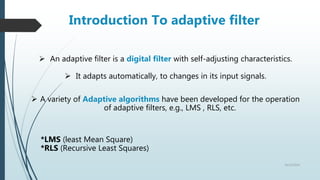
 An adaptive filter is a digital filter with self-adjusting characteristics.
 It adapts automatically, to changes in its input signals.
 A variety of Adaptive algorithms have been developed for the operation
of adaptive filters, e.g., LMS , RLS, etc.
*LMS (least Mean Square)
*RLS (Recursive Least Squares)
Contains 2 main component :
1- Digital filter(with adjustable coefficients).
2- Adaptive Algorithm. 10/13/2016
 We have two input signals into our Adaptive filter:
𝑌𝑘= 𝑆 𝑘+𝑛 𝑘
where
𝒔 𝒌= Desired signal .
𝒏 𝒌= noise.
𝒙 𝒌
A measure of the contaminating signal which is in some way
correlated with 𝑛 𝑘 .
10/13/2016
Noise Cancelling and power
𝑋 𝑘 gives us an estimate of 𝑛 𝑘 ,called it 𝑛 𝑘
^
.
We try to find an estimate of 𝑆 𝑘, by subtracting our best estimate of the
noise signal . Let 𝑆 𝑘
^
be our estimate of the desired signal 𝑆 𝑘 .
𝑆 𝑘
^
= 𝑌𝑘 - 𝑛 𝑘
^
= (𝑆 𝑘 + 𝑛 𝑘) - 𝑛 𝑘
^
10/13/2016
Main objective :
produce Optimum 𝒏 𝒌
^
𝑆 𝑘
^
= 𝑌𝑘 - 𝑛 𝑘
^
= (𝑆 𝑘 + 𝑛 𝑘) - 𝑛 𝑘
^
Theorem: Minimizing the total power at the output of the canceller
maximizes the out signal-to-noise ration.
10/13/2016
Proof
𝑆 𝑘
^
= 𝑌𝑘 - 𝑛 𝑘
^
= (𝑆 𝑘 + 𝑛 𝑘) - 𝑛 𝑘
^
Squaring :
𝑆 𝑘
^2
= 𝑆 𝑘
2
+ (𝑛 𝑘 − 𝑛 𝑘
^
)
2
+ 2𝑆 𝑘(𝑛 𝑘 - 𝑛 𝑘
^
)
Mean :
E ( 𝑆 𝑘
^2
) = E (𝑆 𝑘
2
) + E ( (𝑛 𝑘 − 𝑛 𝑘
^
)
2
) + 2E (𝑆 𝑘(𝑛 𝑘 - 𝑛 𝑘
^
))
E ( 𝑆 𝑘
^2
) = E (𝑆 𝑘
2
) + E ( (𝑛 𝑘 − 𝑛 𝑘
^
)
2
) + 2E (𝑆 𝑘(𝑛 𝑘 - 𝑛 𝑘
^
))
Since the desired signal 𝑆 𝑘 ,is uncorrelated with 𝑛 𝑘 or 𝑛 𝑘
^
,
the last term become zero
E ( 𝑆 𝑘
^2
) = E (𝑆 𝑘
2
) + E ( (𝑛 𝑘 − 𝑛 𝑘
^
)
2
)
E (𝑆 𝑘
2
) represent the signal power. E ( 𝑆 𝑘
^2
) represent the estimate of the
signal power, and + E ( (𝑛 𝑘 − 𝑛 𝑘
^
)
2
) represent the remnant noise power.
The manage of minimize the power of the Noise .
Min E ( 𝑆 𝑘
^2
) = E (𝑆 𝑘
2
) + min E ( (𝑛 𝑘 − 𝑛 𝑘
^
)
2
)
10/13/2016
Applications of Adaptive Filters:
1) Identification
10/13/2016
Used to provide a linear model of an unknown plant.
Applications:
System identification
10/13/2016
Applications of Adaptive Filters:
2) Inverse Modeling
Used to provide an inverse model of an unknown plant
Applications :
Channel Equalization
Used to provide a prediction of the present value of a random signal
Applications :
Signal detection
10/13/2016
Applications of Adaptive Filters:
3) Prediction
Subtracts Noise from Received signal adaptively to improve SNR
10/13/2016
Applications of Adaptive Filters:
4) Echo (Noise) cancellation
A good example to illustrate the principles of adaptive noise cancelling
is the noise removal from the pilot's microphone in the airplane.
Due to the high environmental noise produced by the airplane engines,
the pilot’s voice in the microphone is distorted with a high amount of
noise ,and can be very difficult to understand .
In order to overcome the problem , an adaptive filter can be used.
10/13/2016
Approaches to adaptive filter
10/13/2016
Adaptive
Filtering
Stochastic Gradient
Approach
Least Square
Estimation
(Least Mean Square Algorithms) (Recursive Least Square Algorithm)
LMS
NLMS
TVLMS
VSSNLMS
RLS
FTRL
S
Linear
Non linear Neural Networks
Stochastic Gradient
10/13/2016
Most commonly used type of Adaptive Filters
Define cost function as mean-squared error
Difference between filter output and desired response
Based on the method of steepest descent
Move towards the minimum on the error surface to get to minimum
Requires the gradient of the error surface to be known
Most popular adaptation algorithm is LMS
Derived from steepest descent
Doesn’t require gradient to be know: it is estimated at every iteration
Least-Mean-Square (LMS) Algorithm.
10/13/2016















 
































signal
error
vector
input
tap
parameter
rate
-learning
vector
weight-tapof
valueold
vector
weigth-tapof
valueupdate
In the family of stochastic gradient algorithms
Approximation of the steepest – descent method
Based on the MMSE criterion.(Minimum Mean square Error)
Adaptive process containing two important signals:
1.) Filtering process, producing output signal.
2.) Desired signal (Training sequence)
Adaptive process: Recursive adjustment of filter tap weights
The LMS Algorithm consists of two basic processes that is followed in the adaptive
equalization processes:
Training : It refers to adapting to the training sequence.
Tracking: keeps track of the changing characteristics of the channel.
10/13/2016
LMS Algorithm Steps:
10/13/2016
Filter output
Estimation error
Tap-weight adaptation
     



1
0
*
M
k
k nwknunz
     nzndne 
       neknunwnw kk
*
1  
10/13/2016
Transversal Filter
Stability of LMS:
10/13/2016
 The LMS algorithm is convergent in the mean square if and
only if the step-size parameter satisfy
Here max is the largest Eigen value of the correlation matrix of
the input data.
 More practical test for stability is
 Larger values for step size
Increases adaptation rate (faster adaptation)
Increases residual mean-squared error
max
1
0

 
powersignalinput
1
0  
10/13/2016
LMS – Disadvantage:
 Slow Convergence
 Demands using of training sequence as reference ,thus
decreasing the communication BW.
LMS – Advantage:
 Simplicity of implementation
 Not neglecting the noise like Zero forcing equalizer
 Stable and robust performance against different signal
conditions
The design of a Wiener filter requires a priori information about the statistics of the
data to be processed.
The filter is optimum only when the statistical characteristics of the input data match
the a priori information on which the design of the filter is based.
10/13/2016
Wiener filter
Many adaptive algorithms can be viewed as approximation to the discrete
Wiener filter.
Tries to minimize the mean of the square of the error
(Least Mean Square)
Assuming an FIR filter structure with N coefficient (weights) the output signal is given
by:
10/13/2016
Where 𝐗 𝐤 is the vector correlated with the noise at the 𝐾 𝑡ℎ sample and W is the set of
adjustable weights.
Squaring the error:
10/13/2016
(The N-length Cross-Correlation Vector)
(The N * N autocorrelation matrix).
Mean :
Where P = E ( 𝑌𝐴 𝑋 𝐾)
And R = E ( 𝑋 𝑘 𝑋 𝑘
𝑇
)
The mean square
10/13/2016
The wiener-Hopf solution
10/13/2016
Setting gradient to zero
𝑾 𝒐𝒑𝒕 =𝑹−𝟏 P
Where P = E ( 𝒀 𝑨 𝑿 𝑲)
And R = E ( 𝑿 𝒌 𝑿 𝒌
𝑻
)
Issues with the wiener – Hopf solution
10/13/2016
1. Requires knowledge of R and P , nither of which are known
before-hand.
2. Matrix inversion is expensive (O(𝑛3))
3. If the signals are non-stionary. Then both R and P will
Change with time , and so 𝑊𝑜𝑝𝑡 will have to be computed
repeatedly.
The windrow-Hopf LMS algorithm
10/13/2016
Base on the the steepest descent algorithm
Where
U determines Stability and rate convergence.
 If u is too large, we observe too much fluctuation.
 If u is too small, rate of convergence too slow.
Least Square Estimation
10/13/2016
Recursive Least Square (RLS) Algorithm
10/13/2016
Recursive Least Square (RLS) Algorithm
10/13/2016
Gama (typically between 0.98 and 1) is referred to as the
“forgetting factor”.
The previous samples contribute less and less to the new
weights:
when Y=1, we have “infinite memory” and this weighting
scheme reduce to exract Least Squares solution.
10/13/2016
Comparison against LMS
10/13/2016
 RLS has rapid rate convergence, compared to LMS.
 RLS is computationally more expensive than LMS.
10/13/2016
Thank YOU ^_^
10/13/2016

Adaptive filter

  • 1.
  • 2.
    “Adaptive filter Theory“ By Simon Haykin ” Adaptive filter “ By B.Farhang boroujeny ” Adaptive Linear & Nonlinear Filters “ By (Frank) XiangYang Gao 10/13/2016 References:
  • 3.
    10/13/2016 Overview Before we startwe must understand some concept :  The term filter is a “black box” that takes an input signal ,processes it, and then returns an output signal that in some way modifies the input. For example, if the input signal is noisy, then one would want a filter that removes noise, but otherwise leaves the signal unchanged.  we may use a filter to perform three basic information-processing tasks: 1. Filtering, which means the extraction of information about a quantity of interest at time t by using data measured up to and including time t.
  • 4.
    10/13/2016 2. Smoothing, whichdiffers from filtering in that information about the quantity of interest need not be available at time t , This means that in the case of smoothing there is a delay in producing the result of interest. 3. Prediction, which is the forecasting side of information processing. The aim here is to derive information about what the quantity of interest will be like at some time t + T in the future, for some z > 0, by using data measured up to and including time t.
  • 5.
    10/13/2016 Filter linear Non linear We may classify filters into linear and nonlinear. A filter is said to be linear if the 1) filtered 2) smoothed 3) predicted quantity at the output of the device is a linear function of the observations applied w the filter input. Otherwise, the filter is nonlinear.
  • 6.
    Fixed versus AdaptiveFilter Design 10/13/2016 W0 , W1 , W2 ,…….. Wn-1Fixed Determine the values of the coefficients of the digital filter that meet the desired specifications and the values are not changed once they are implemented The coefficient values are not fixed. They are adjusted to optimize some measure of the filter performance using incoming input data and error. W0(n) , W1(n) , W2(N),….Wn-1(N)Adaptive
  • 7.
     The figureshows a filter emphasizing the way it is used in typical problems. The filter is used to reshape certain input signals in such a way that its output is a good estimate of the given desired signal. 10/13/2016 Introduction To adaptive filter Filter (A.F)Input signal Output signal Desired signal Error signal+
  • 8.
    Introduction To adaptivefilter 10/13/2016  An adaptive filter is a digital filter with self-adjusting characteristics.  It adapts automatically, to changes in its input signals.  A variety of Adaptive algorithms have been developed for the operation of adaptive filters, e.g., LMS , RLS, etc. *LMS (least Mean Square) *RLS (Recursive Least Squares)
  • 9.
    Contains 2 maincomponent : 1- Digital filter(with adjustable coefficients). 2- Adaptive Algorithm. 10/13/2016
  • 10.
     We havetwo input signals into our Adaptive filter: 𝑌𝑘= 𝑆 𝑘+𝑛 𝑘 where 𝒔 𝒌= Desired signal . 𝒏 𝒌= noise. 𝒙 𝒌 A measure of the contaminating signal which is in some way correlated with 𝑛 𝑘 . 10/13/2016 Noise Cancelling and power
  • 11.
    𝑋 𝑘 givesus an estimate of 𝑛 𝑘 ,called it 𝑛 𝑘 ^ . We try to find an estimate of 𝑆 𝑘, by subtracting our best estimate of the noise signal . Let 𝑆 𝑘 ^ be our estimate of the desired signal 𝑆 𝑘 . 𝑆 𝑘 ^ = 𝑌𝑘 - 𝑛 𝑘 ^ = (𝑆 𝑘 + 𝑛 𝑘) - 𝑛 𝑘 ^ 10/13/2016 Main objective : produce Optimum 𝒏 𝒌 ^
  • 12.
    𝑆 𝑘 ^ = 𝑌𝑘- 𝑛 𝑘 ^ = (𝑆 𝑘 + 𝑛 𝑘) - 𝑛 𝑘 ^ Theorem: Minimizing the total power at the output of the canceller maximizes the out signal-to-noise ration. 10/13/2016 Proof 𝑆 𝑘 ^ = 𝑌𝑘 - 𝑛 𝑘 ^ = (𝑆 𝑘 + 𝑛 𝑘) - 𝑛 𝑘 ^ Squaring : 𝑆 𝑘 ^2 = 𝑆 𝑘 2 + (𝑛 𝑘 − 𝑛 𝑘 ^ ) 2 + 2𝑆 𝑘(𝑛 𝑘 - 𝑛 𝑘 ^ ) Mean : E ( 𝑆 𝑘 ^2 ) = E (𝑆 𝑘 2 ) + E ( (𝑛 𝑘 − 𝑛 𝑘 ^ ) 2 ) + 2E (𝑆 𝑘(𝑛 𝑘 - 𝑛 𝑘 ^ ))
  • 13.
    E ( 𝑆𝑘 ^2 ) = E (𝑆 𝑘 2 ) + E ( (𝑛 𝑘 − 𝑛 𝑘 ^ ) 2 ) + 2E (𝑆 𝑘(𝑛 𝑘 - 𝑛 𝑘 ^ )) Since the desired signal 𝑆 𝑘 ,is uncorrelated with 𝑛 𝑘 or 𝑛 𝑘 ^ , the last term become zero E ( 𝑆 𝑘 ^2 ) = E (𝑆 𝑘 2 ) + E ( (𝑛 𝑘 − 𝑛 𝑘 ^ ) 2 ) E (𝑆 𝑘 2 ) represent the signal power. E ( 𝑆 𝑘 ^2 ) represent the estimate of the signal power, and + E ( (𝑛 𝑘 − 𝑛 𝑘 ^ ) 2 ) represent the remnant noise power. The manage of minimize the power of the Noise . Min E ( 𝑆 𝑘 ^2 ) = E (𝑆 𝑘 2 ) + min E ( (𝑛 𝑘 − 𝑛 𝑘 ^ ) 2 ) 10/13/2016
  • 14.
    Applications of AdaptiveFilters: 1) Identification 10/13/2016 Used to provide a linear model of an unknown plant. Applications: System identification
  • 15.
    10/13/2016 Applications of AdaptiveFilters: 2) Inverse Modeling Used to provide an inverse model of an unknown plant Applications : Channel Equalization
  • 16.
    Used to providea prediction of the present value of a random signal Applications : Signal detection 10/13/2016 Applications of Adaptive Filters: 3) Prediction
  • 17.
    Subtracts Noise fromReceived signal adaptively to improve SNR 10/13/2016 Applications of Adaptive Filters: 4) Echo (Noise) cancellation
  • 18.
    A good exampleto illustrate the principles of adaptive noise cancelling is the noise removal from the pilot's microphone in the airplane. Due to the high environmental noise produced by the airplane engines, the pilot’s voice in the microphone is distorted with a high amount of noise ,and can be very difficult to understand . In order to overcome the problem , an adaptive filter can be used. 10/13/2016
  • 19.
    Approaches to adaptivefilter 10/13/2016 Adaptive Filtering Stochastic Gradient Approach Least Square Estimation (Least Mean Square Algorithms) (Recursive Least Square Algorithm) LMS NLMS TVLMS VSSNLMS RLS FTRL S Linear Non linear Neural Networks
  • 20.
    Stochastic Gradient 10/13/2016 Most commonlyused type of Adaptive Filters Define cost function as mean-squared error Difference between filter output and desired response Based on the method of steepest descent Move towards the minimum on the error surface to get to minimum Requires the gradient of the error surface to be known Most popular adaptation algorithm is LMS Derived from steepest descent Doesn’t require gradient to be know: it is estimated at every iteration
  • 21.
    Least-Mean-Square (LMS) Algorithm. 10/13/2016                                                 signal error vector input tap parameter rate -learning vector weight-tapof valueold vector weigth-tapof valueupdate In the family of stochastic gradient algorithms Approximation of the steepest – descent method Based on the MMSE criterion.(Minimum Mean square Error) Adaptive process containing two important signals: 1.) Filtering process, producing output signal. 2.) Desired signal (Training sequence)
  • 22.
    Adaptive process: Recursiveadjustment of filter tap weights The LMS Algorithm consists of two basic processes that is followed in the adaptive equalization processes: Training : It refers to adapting to the training sequence. Tracking: keeps track of the changing characteristics of the channel. 10/13/2016
  • 23.
    LMS Algorithm Steps: 10/13/2016 Filteroutput Estimation error Tap-weight adaptation          1 0 * M k k nwknunz      nzndne         neknunwnw kk * 1  
  • 24.
  • 25.
    Stability of LMS: 10/13/2016 The LMS algorithm is convergent in the mean square if and only if the step-size parameter satisfy Here max is the largest Eigen value of the correlation matrix of the input data.  More practical test for stability is  Larger values for step size Increases adaptation rate (faster adaptation) Increases residual mean-squared error max 1 0    powersignalinput 1 0  
  • 26.
    10/13/2016 LMS – Disadvantage: Slow Convergence  Demands using of training sequence as reference ,thus decreasing the communication BW. LMS – Advantage:  Simplicity of implementation  Not neglecting the noise like Zero forcing equalizer  Stable and robust performance against different signal conditions
  • 27.
    The design ofa Wiener filter requires a priori information about the statistics of the data to be processed. The filter is optimum only when the statistical characteristics of the input data match the a priori information on which the design of the filter is based. 10/13/2016 Wiener filter Many adaptive algorithms can be viewed as approximation to the discrete Wiener filter. Tries to minimize the mean of the square of the error (Least Mean Square)
  • 28.
    Assuming an FIRfilter structure with N coefficient (weights) the output signal is given by: 10/13/2016 Where 𝐗 𝐤 is the vector correlated with the noise at the 𝐾 𝑡ℎ sample and W is the set of adjustable weights.
  • 29.
    Squaring the error: 10/13/2016 (TheN-length Cross-Correlation Vector) (The N * N autocorrelation matrix). Mean : Where P = E ( 𝑌𝐴 𝑋 𝐾) And R = E ( 𝑋 𝑘 𝑋 𝑘 𝑇 )
  • 30.
  • 31.
    The wiener-Hopf solution 10/13/2016 Settinggradient to zero 𝑾 𝒐𝒑𝒕 =𝑹−𝟏 P Where P = E ( 𝒀 𝑨 𝑿 𝑲) And R = E ( 𝑿 𝒌 𝑿 𝒌 𝑻 )
  • 32.
    Issues with thewiener – Hopf solution 10/13/2016 1. Requires knowledge of R and P , nither of which are known before-hand. 2. Matrix inversion is expensive (O(𝑛3)) 3. If the signals are non-stionary. Then both R and P will Change with time , and so 𝑊𝑜𝑝𝑡 will have to be computed repeatedly.
  • 33.
    The windrow-Hopf LMSalgorithm 10/13/2016 Base on the the steepest descent algorithm Where U determines Stability and rate convergence.  If u is too large, we observe too much fluctuation.  If u is too small, rate of convergence too slow.
  • 34.
  • 35.
    Recursive Least Square(RLS) Algorithm 10/13/2016
  • 36.
    Recursive Least Square(RLS) Algorithm 10/13/2016
  • 37.
    Gama (typically between0.98 and 1) is referred to as the “forgetting factor”. The previous samples contribute less and less to the new weights: when Y=1, we have “infinite memory” and this weighting scheme reduce to exract Least Squares solution. 10/13/2016
  • 38.
    Comparison against LMS 10/13/2016 RLS has rapid rate convergence, compared to LMS.  RLS is computationally more expensive than LMS.
  • 39.
  • 40.