Downloaded 45 times


![Slide 29
A (1 - ) 100% confidence interval for , the mean of population i:
i
a m
a
a
where t is the value of the distribution with ) degrees of
freedom that cuts off a right - tailed area of
2
.
2
a
x
t
MSE
n
i
i
±
2
t (n- r
x t
MSE
n
x x
i
i
i i
± = ± = ±
± =
± =
± =
± =
± =
a
2
196
504 39
40
6 96
89 6 96 82 04 95 96]
75 6 96 68 04 81 96]
73 6 96 66 04 79 96]
91 6 96 84 04 97 96]
85 6 96 78 04 91 96]
.
.
.
. [ . , .
. [ . , .
. [ . , .
. [ . , .
. [ . , .
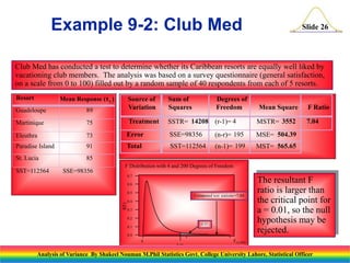
Resort Mean Response (x i)
Guadeloupe 89
Martinique 75
Eleuthra 73
Paradise Island 91
St. Lucia 85
SST = 112564 SSE = 98356
ni = 40 n = (5)(40) = 200
MSE = 504.39
Confidence Intervals for
Population Means
Analysis of Variance By Shakeel Nouman M.Phil Statistics Govt. College University Lahore, Statistical Officer](https://image.slidesharecdn.com/analysisofvariance-140129013602-phpapp02/85/Analysis-of-variance-29-320.jpg)

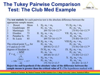
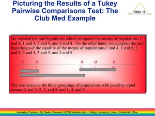


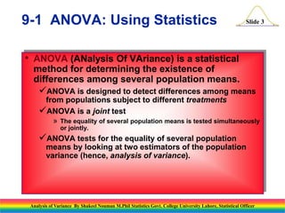
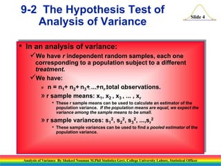
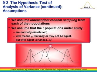
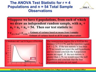
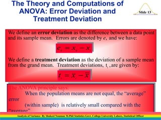
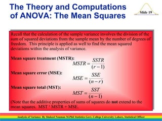
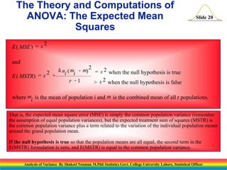
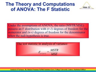
This document presents an analysis of variance (ANOVA) methodology, explaining its purpose in detecting differences among several population means through statistical tests. It outlines key concepts such as the test statistic, hypotheses, and the importance of understanding the roles of variation within and between samples. Additionally, it discusses computation techniques including sums of squares and degrees of freedom, crucial for implementing ANOVA effectively in statistical analyses.