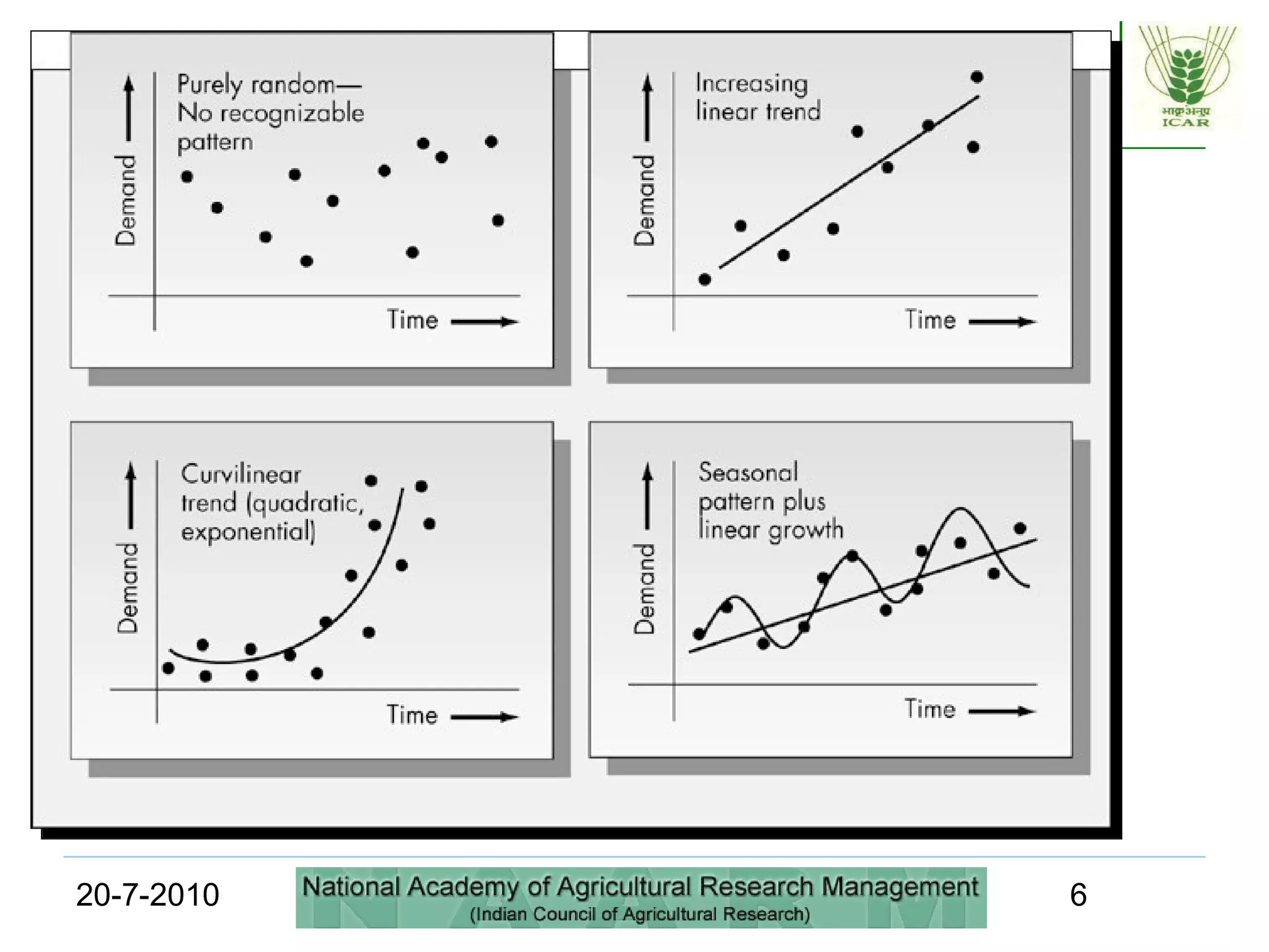
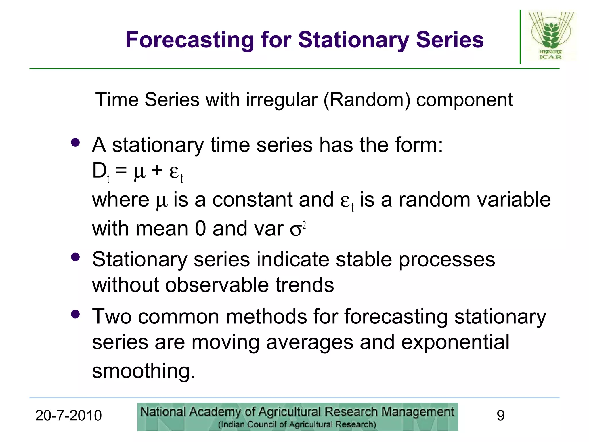
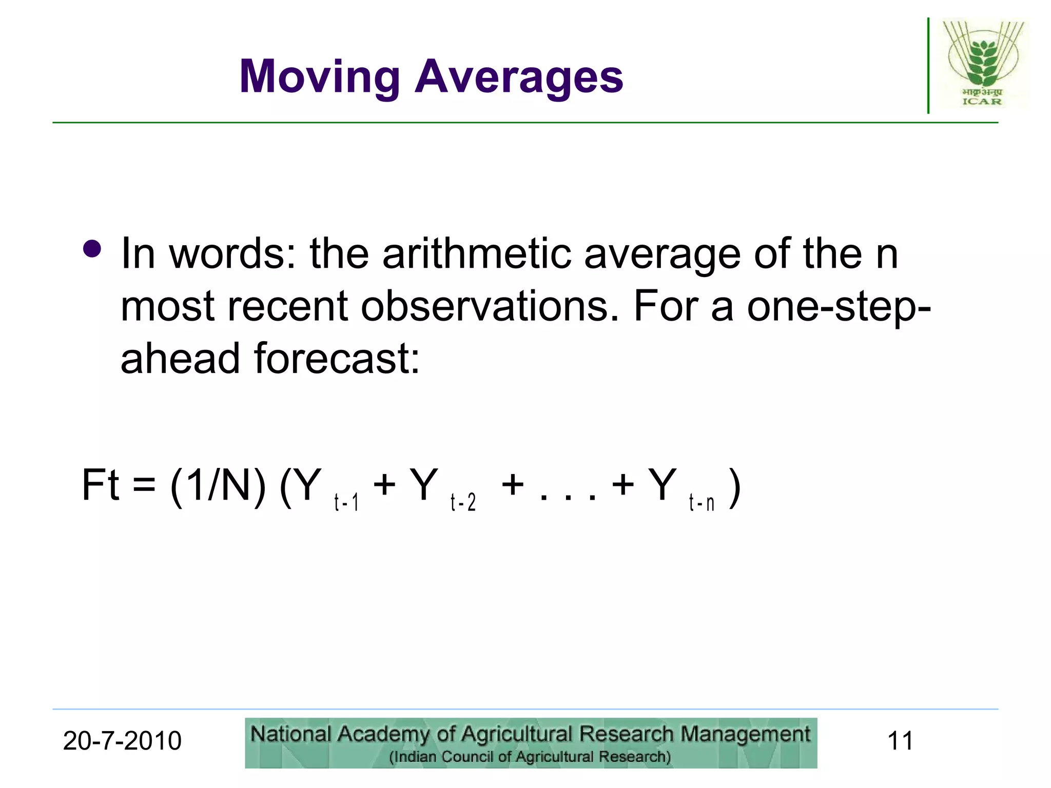
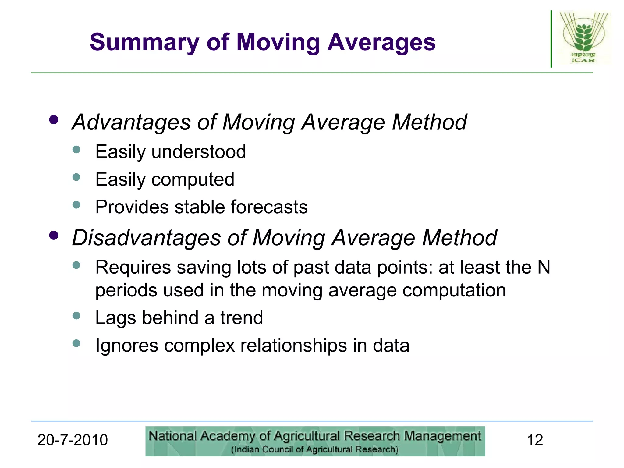
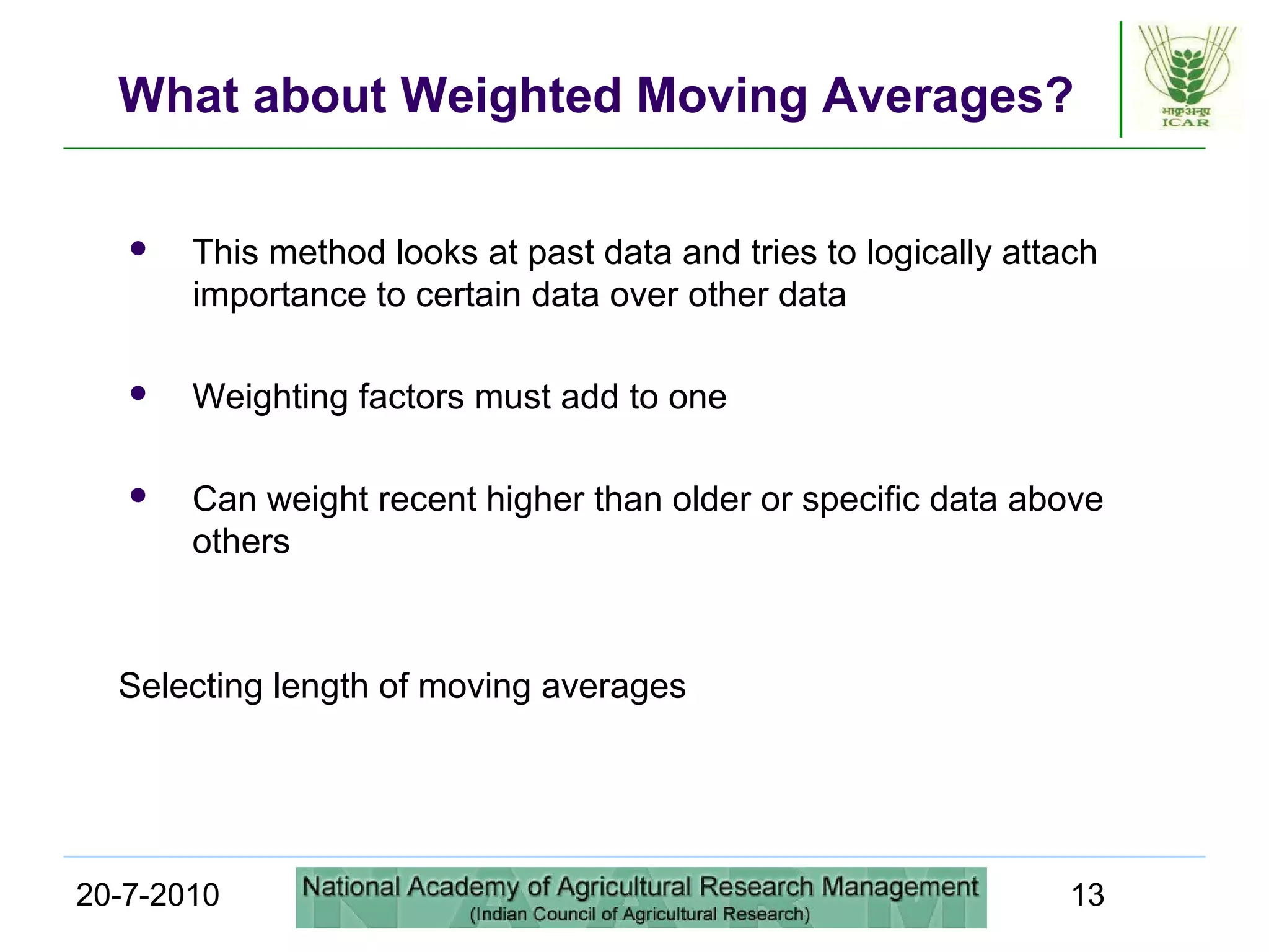
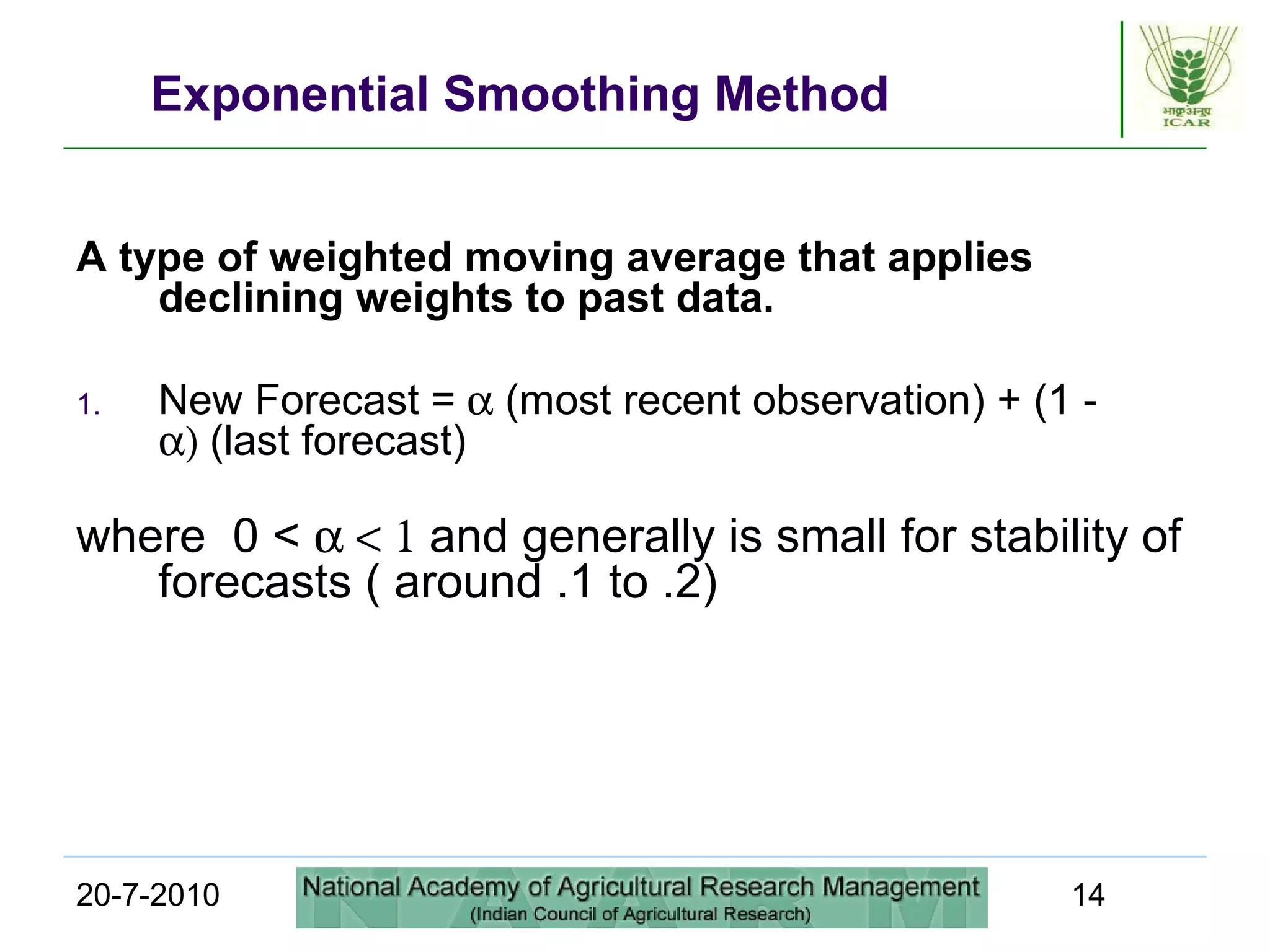
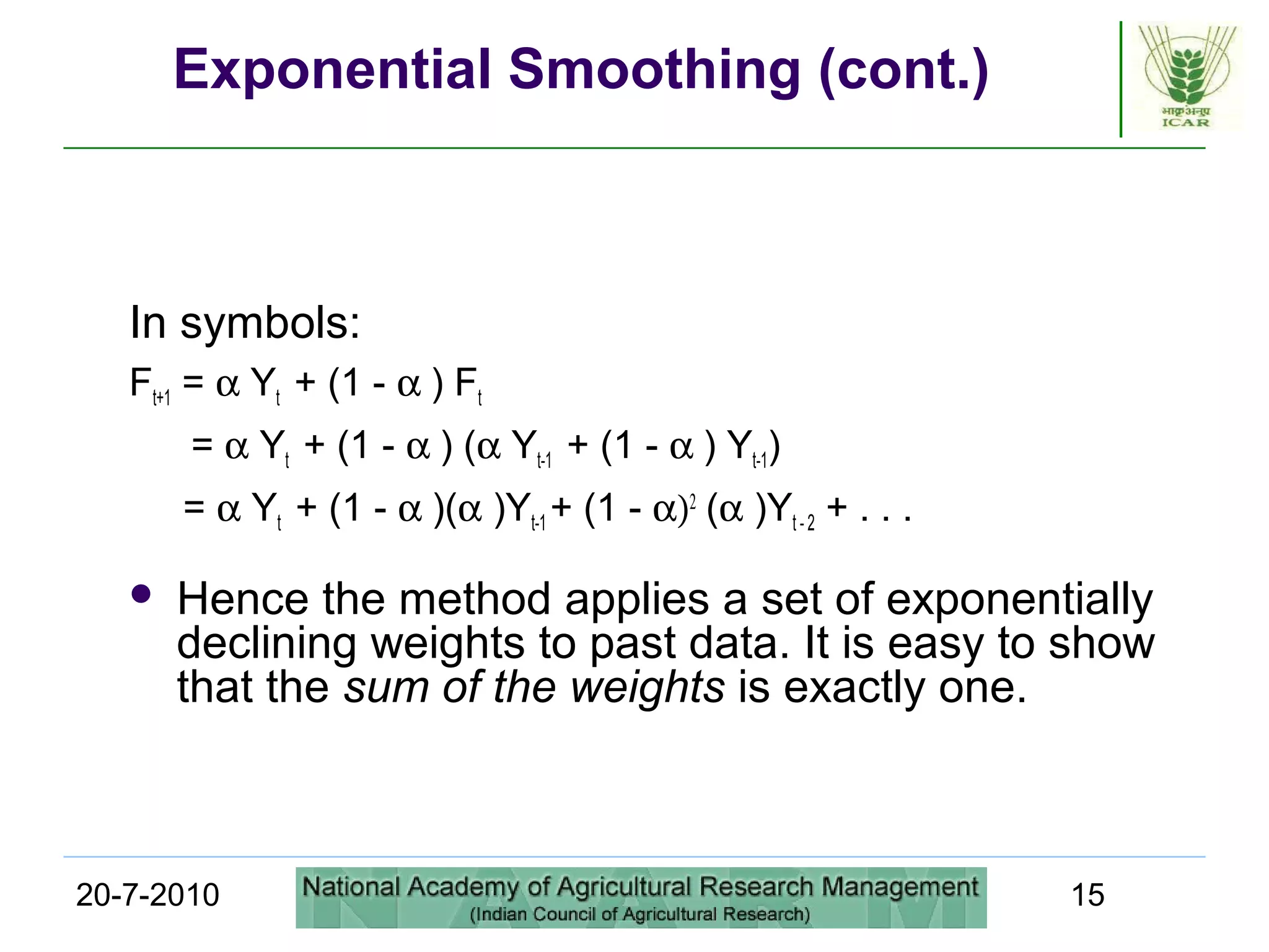
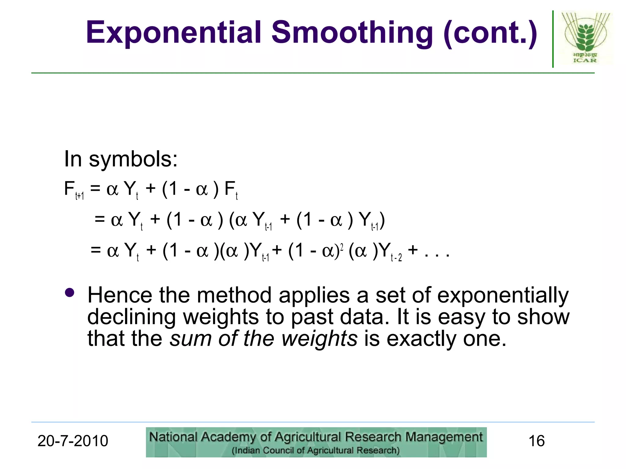
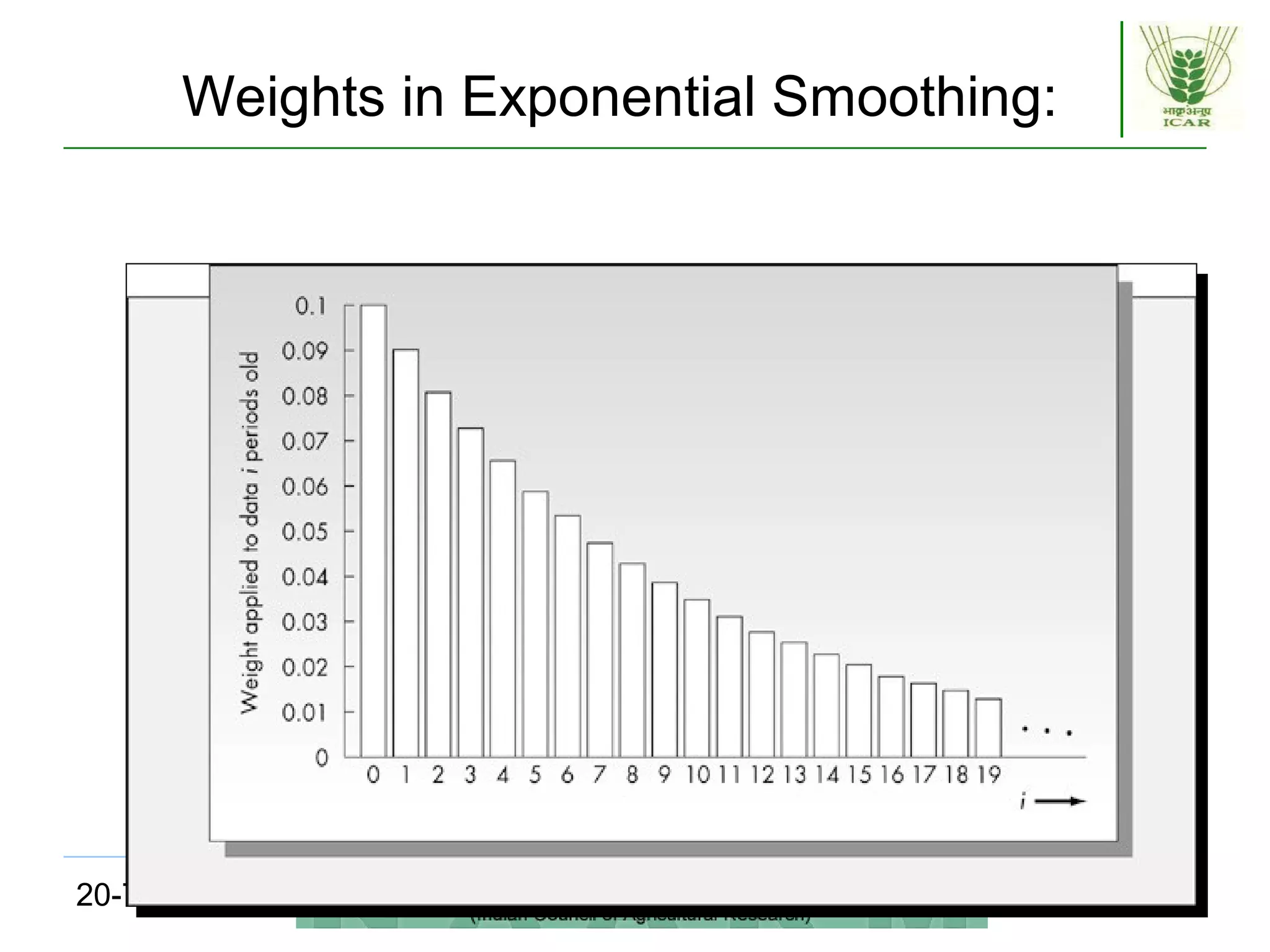
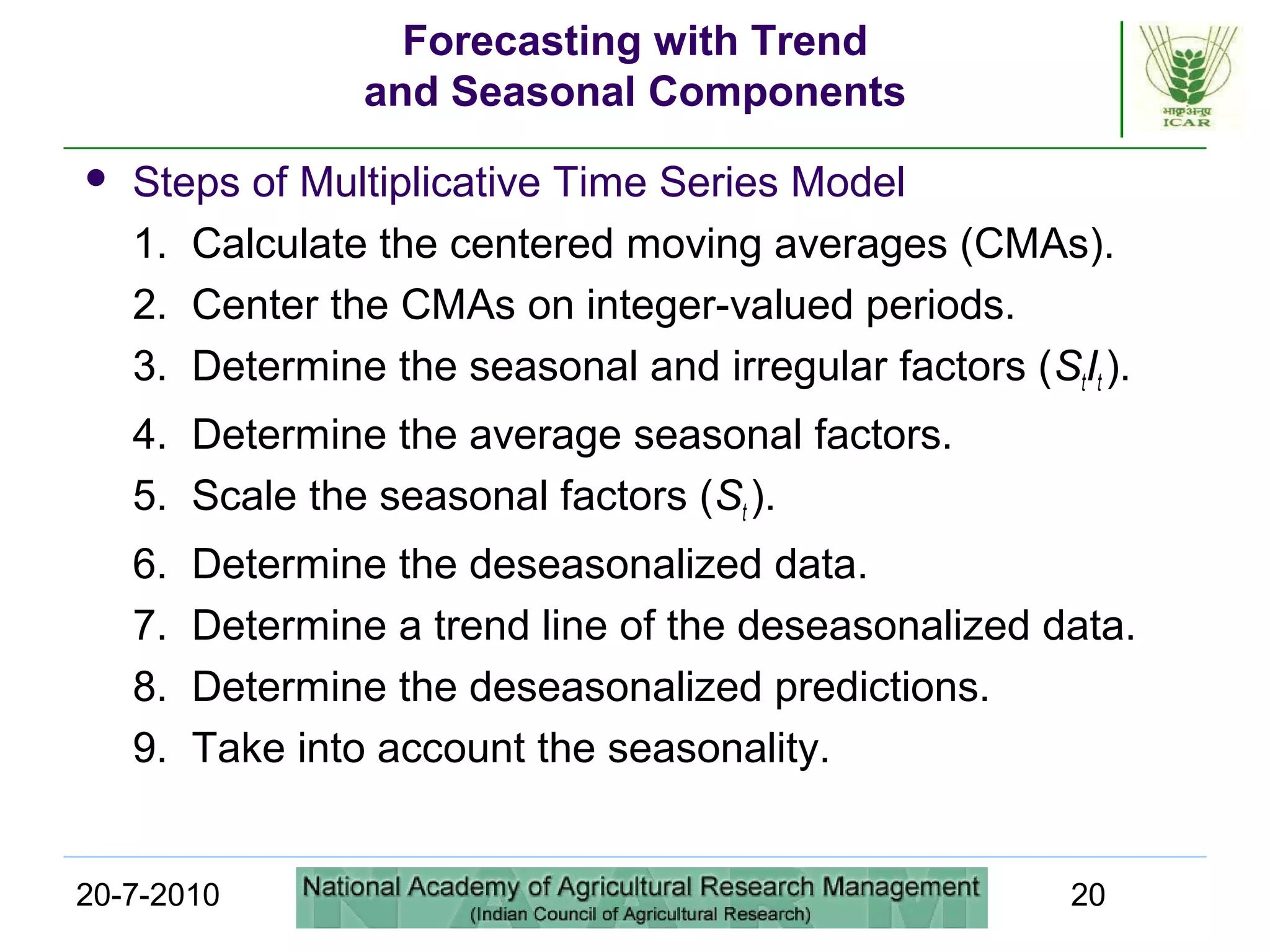
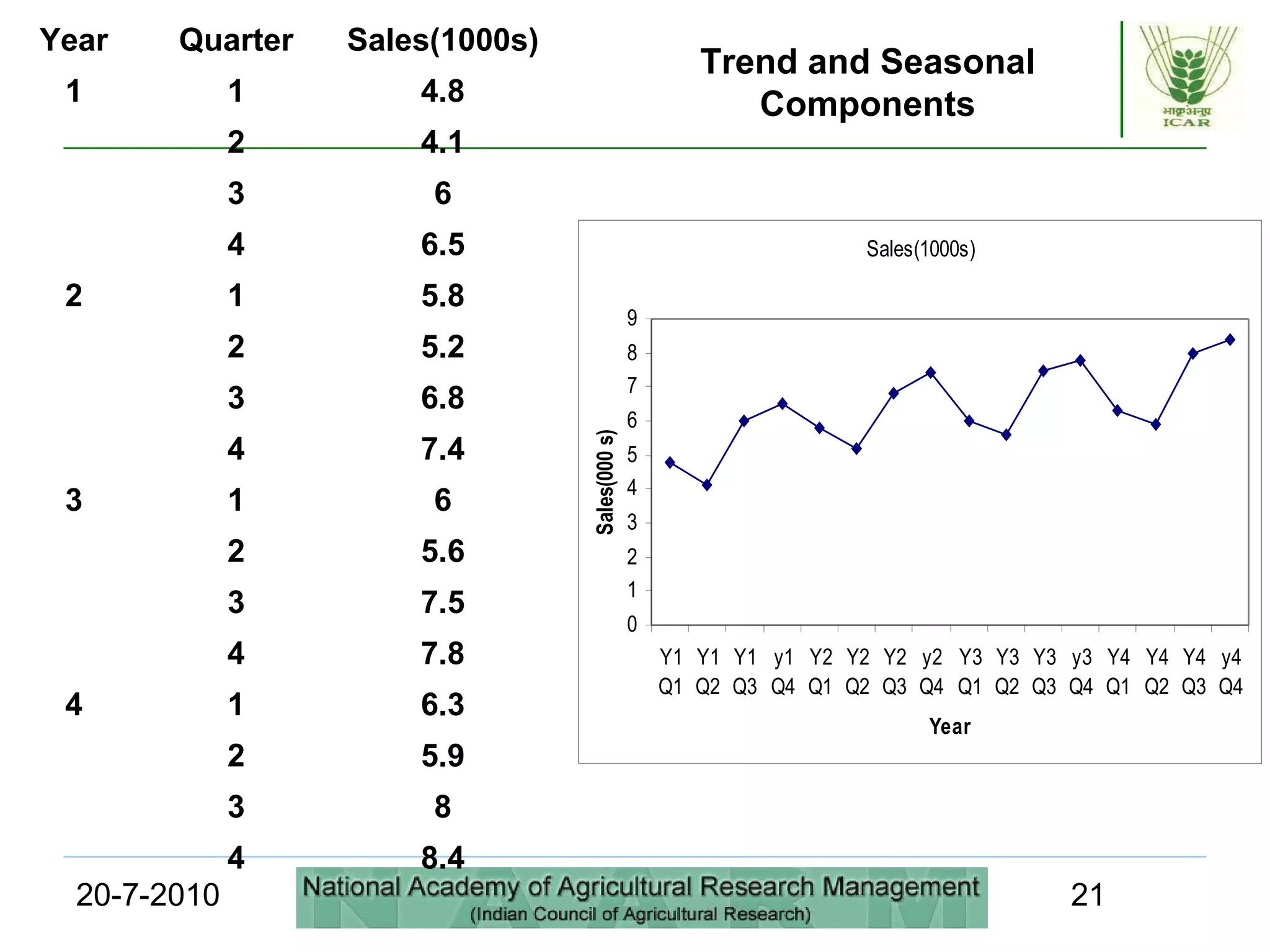
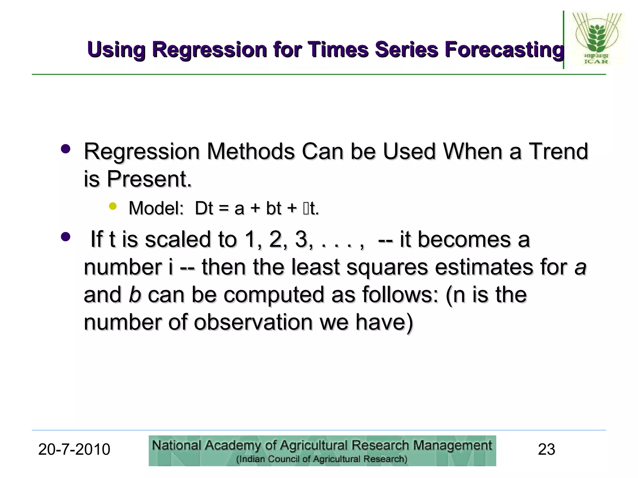
This document discusses quantitative forecasting methods, including time series and causal models. It covers key time series components like trend, seasonality, and cycles. Three main time series methods are described: smoothing, trend projection, and trend projection adjusted for seasonal influence. Moving averages and exponential smoothing are explained as common techniques for forecasting stationary time series. The document also covers decomposing a time series into trend, seasonal, and irregular components. Regression methods are mentioned as another approach when a trend is present in the data.

1. Quantitative Methods for Business
PGDMA-624
Time Series Forecasting
Note: Adapted from “Quantitative Methods for Business
by Anderson et all.

2. 20-7-2010 2
Quantitative Approaches to
Forecasting
 Quantitative methods are based on an analysis of
historical data concerning one or more time series.
 A time series is a set of observations measured at
successive points in time or over successive periods
of time.
 If the historical data used are restricted to past values
of the series that we are trying to forecast, the
procedure is called a time series method.
 If the historical data used involve other time series
that are believed to be related to the time series that
we are trying to forecast, the procedure is called a
causal method.

3. 20-7-2010 3
Time Series Methods
 Three time series methods are:
 smoothing
 trend projection
 trend projection adjusted for seasonal influence
 Two primary methods: causal models and time series methods
Causal Models (Regression Models)
Let Y be the quantity to be forecasted and (X1,
X2, . . . , Xn) are n variables that have predictive power for Y. A causal
model is Y = f (X1, X2, . . . , Xn).
A typical relationship is a linear one:
Y = a0 + a1X1 + . . . + an Xn

4. 20-7-2010 4
Time Series Methods
 A time series is just collection of past values of
the variable being predicted. Also known as
naïve methods. Goal is to isolate patterns in past
data. (See Figures on following pages)
Components of Time series
 Trend
 Seasonality
 Cycles
 Irregular Component or Randomness

5. 20-7-2010 5
Components of a Time Series
 The trend component accounts for the gradual shifting
of the time series over a long period of time.
 Any regular pattern of sequences of values above and
below the trend line is attributable to the cyclical
component of the series.
 The seasonal component of the series accounts for
regular patterns of variability within certain time periods,
such as over a year.
 The irregular component of the series is caused by
short-term, unanticipated and non-recurring factors that
affect the values of the time series. One cannot attempt
to predict its impact on the time series in advance.

6. 20-7-2010 6

7. 20-7-2010 7
Notation Conventions
 Let Y1, Y2, . . . Yn, . . . be the past values of the series to be
predicted (demands?). If we are making a forecast during period
t (for the future), assume we have observed Yt , Yt-1 etc.
 Let Ft = forecast made in period t
Models of Time Series
Additive Model: Y= S+T+C+I
Multiplicative Model : Y =S.T.C.I

8. 20-7-2010 8
Evaluation of Forecasts
 The forecast error in period t, et, is the difference
between the forecast for demand in period t and the
actual value of demand in t.
 For one step ahead forecast: et = Yt – Ft
 To evaluate Forecasting accuracy we develop a chart
of Forecasting errors using:
Mean Square error =MSE = (1/n) Σ ei
2
Root Mean Square error = RMSE = √MSE
Mean absolute Deviation: MAD = (1/n) Σ | e i |

9. 20-7-2010 9
Forecasting for Stationary Series
 A stationary time series has the form:
Dt = µ + εt
where µ is a constant and εt is a random variable
with mean 0 and var σ2
 Stationary series indicate stable processes
without observable trends
 Two common methods for forecasting stationary
series are moving averages and exponential
smoothing.
Time Series with irregular (Random) component

10. 20-7-2010 10
Week
Sales (1000
of
gallons)
1 17
2 21
3 19
4 23
5 18
6 16
7 20
8 18
9 22
10 20
11 15
12 22
Example
Sales (1000 of gallons)
0
5
10
15
20
25
1 2 3 4 5 6 7 8 9 10 11 12
Week
Sales(1000sofones)

11. 20-7-2010 11
Moving Averages
 In words: the arithmetic average of the n
most recent observations. For a one-step-
ahead forecast:
Ft = (1/N) (Y t - 1 + Y t - 2 + . . . + Y t - n )

12. 20-7-2010 12
Summary of Moving Averages
 Advantages of Moving Average Method
 Easily understood
 Easily computed
 Provides stable forecasts
 Disadvantages of Moving Average Method
 Requires saving lots of past data points: at least the N
periods used in the moving average computation
 Lags behind a trend
 Ignores complex relationships in data

13. 20-7-2010 13
What about Weighted Moving Averages?
 This method looks at past data and tries to logically attach
importance to certain data over other data
 Weighting factors must add to one
 Can weight recent higher than older or specific data above
others
Selecting length of moving averages

14. 20-7-2010 14
Exponential Smoothing Method
A type of weighted moving average that applies
declining weights to past data.
1. New Forecast = α (most recent observation) + (1 -
α) (last forecast)
where 0 < α < 1 and generally is small for stability of
forecasts ( around .1 to .2)

15. 20-7-2010 15
Exponential Smoothing (cont.)
In symbols:
Ft+1 = α Yt + (1 - α ) Ft
= α Yt + (1 - α ) (α Yt-1 + (1 - α ) Yt-1)
= α Yt + (1 - α )(α )Yt-1 + (1 - α)2
(α )Yt - 2 + . . .
 Hence the method applies a set of exponentially
declining weights to past data. It is easy to show
that the sum of the weights is exactly one.

16. 20-7-2010 16
Exponential Smoothing (cont.)
In symbols:
Ft+1 = α Yt + (1 - α ) Ft
= α Yt + (1 - α ) (α Yt-1 + (1 - α ) Yt-1)
= α Yt + (1 - α )(α )Yt-1 + (1 - α)2
(α )Yt - 2 + . . .
 Hence the method applies a set of exponentially
declining weights to past data. It is easy to show
that the sum of the weights is exactly one.

17. 20-7-2010 17
Weights in Exponential Smoothing:

18. 20-7-2010 18
Comparison of MA and ES
 Similarities
 Both methods are appropriate for stationary
series
 Both methods depend on a single parameter
 Both methods lag behind a trend

19. 20-7-2010 19
Comparison of MA and ES
 Differences
 ES carries all past history (forever!)
 MA eliminates “bad” data after N periods
 MA requires all N past data points to compute
new forecast estimate while ES only requires
last forecast and last observation of ‘demand’
to continue

20. 20-7-2010 20
Forecasting with Trend
and Seasonal Components
 Steps of Multiplicative Time Series Model
1. Calculate the centered moving averages (CMAs).
2. Center the CMAs on integer-valued periods.
3. Determine the seasonal and irregular factors (StIt ).
4. Determine the average seasonal factors.
5. Scale the seasonal factors (St ).
6. Determine the deseasonalized data.
7. Determine a trend line of the deseasonalized data.
8. Determine the deseasonalized predictions.
9. Take into account the seasonality.

21. 20-7-2010 21
Year Quarter Sales(1000s)
1 1 4.8
2 4.1
3 6
4 6.5
2 1 5.8
2 5.2
3 6.8
4 7.4
3 1 6
2 5.6
3 7.5
4 7.8
4 1 6.3
2 5.9
3 8
4 8.4
Trend and Seasonal
Components
Sales(1000s)
0
1
2
3
4
5
6
7
8
9
Y1
Q1
Y1
Q2
Y1
Q3
y1
Q4
Y2
Q1
Y2
Q2
Y2
Q3
y2
Q4
Y3
Q1
Y3
Q2
Y3
Q3
y3
Q4
Y4
Q1
Y4
Q2
Y4
Q3
y4
Q4
Year
Sales(000s)

22. 20-7-2010 22
Calculating Seasonal Indices
De seasonalizing time series
Estimating Trend
Forecasting by adjusting seasonal variations
Fore casting

23. 20-7-2010 23
Using Regression for Times Series ForecastingUsing Regression for Times Series Forecasting
 Regression Methods Can be Used When a TrendRegression Methods Can be Used When a Trend
is Present.is Present.
 Model: Dt = a + bt +Model: Dt = a + bt + tt..
 If t is scaled to 1, 2, 3, . . . , -- it becomes aIf t is scaled to 1, 2, 3, . . . , -- it becomes a
number i -- then the least squares estimates fornumber i -- then the least squares estimates for aa
andand bb can be computed as follows: (n is thecan be computed as follows: (n is the
number of observation we have)number of observation we have)