econometrics project PG1 2015-16

2015
JADAVPUR UNIVERSITY
DEPARTMENT OF ECONOMICSPG I
SEMESTER II
16-Apr-15
TIME SERIES ANALYSIS OF REAL
GDP AND SHARE OF
AGRICULTURE AND ALLIED
SECTOR
ANKITA MONDAL-001400302024
SAYANTAN BAIDYA-001400302042
SOUMI BHATTACHARYA-001400302043
DEEPANWITA SAHA-001400302045
KRISHNENDU HALDER-001400302055

TIME SERIES ANALYSIS OF REAL GDP AND SHARE OF AGRICULTURE AND
ALLIED SECTOR 2015
2 | P a g e
CONTENTS
MODEL JUSTIFICATION………………………………………………...14
3
4
5
6
31
30

ALLIED SECTOR 2015
3 | P a g e
ACKNOWLEDGEMENT
We are grateful to the faculty of Department of Economics (Jadavpur University) for
their unwavering support and cooperation. Working on this project has given us the
opportunity to gather immense knowledge
regarding econometric tools and economic analysis that will surely benefit us
significantly in our careers in the future. We thank our professor Dr. Arpita Dhar
immensely for setting us this task of preparing and presenting this project. We are
extremely grateful and thankful to her for her tireless guidance without which it
would not have been possible for us to make progress in our endeavour. We also
take this opportunity to thank our department for providing us with a functioning
computer laboratory and library facilities which helped us to fulfil all our needs
regarding our project. Moreover, we are also grateful to our friends and families for
their constant support and help.

ALLIED SECTOR 2015
4 | P a g e
ABSTRACT
This paper is an endeavor to examine the relationship between the total GDP of INDIA & GDP
in agriculture and allied sector in India. Empirical evidence is obtained by applying the Time
Series Analysis on the annual data collected from the MINISTRY OF STATISTICS AND
PROGRAMME IMPLEMENTATION. Using Box Jenkins Approach, Unit Root test, we derive
results which show that there is no long run significant and positive relation between total
GDP of INDIA & GDP in agriculture and allied sector.
Keywords : Economics liberalization, agricultural reform, sectoral reform India ,time series,
inflation, growth,
JEL Classification : O1, O5, Q2,c22, h62, o47

ALLIED SECTOR 2015
5 | P a g e
INTRODUCTION
Time series refers to a sequence of observations following each other in time, where
adjacent observations are correlated. This can be used to model, simulate, and forecast
behavior for a system. Time series models are frequently used in fields such as economics,
finance, biology, and engineering.
The Wolfram Language provides a full suite of time series functionality, including
standard models such as MA, AR, and ARMA, as well as several extensions. Time series
models can be simulated, estimated from data, and used to produce forecasts of future
behavior.
The Indian agriculture sector accounts for 18 per cent of India's gross domestic product
(GDP) and employs just a little less than 50 per cent of the country's workforce. This sector
has made considerable progress in the last few decades with its large resources of land,
water and sunshine. India is presently the world's largest producer of pulses and the second
largest producer of rice and wheat.
The country is also the largest producer, consumer and exporter of spices and spice
products in the world and overall in farm and agriculture outputs, it is ranked second. From
canned, dairy, processed, frozen food to fisheries, meat, poultry, and food grains, the Indian
agro industry has plenty of areas to choose for business.
The Department of Agriculture and Cooperation under the Ministry of Agriculture is the
nodal organisation responsible for the development of the agriculture sector in India. Under
it, several other bodies such as the National Dairy Development Board (NDDB) work for
the development of the other allied agricultural sectors.
“Agriculture is not crop production as popular belief holds - it's the production of food and
fiber from the world's land and waters. Without agriculture it is not possible to have a city,
stock market, banks, university, church or army. Agriculture is the foundation of
civilization and any stable economy.”
By Allan Savory

ALLIED SECTOR 2015
6 | P a g e
ECONOMETRIC THEORY-TIME SERIES
ANALYSIS
A time series is a sequence of data points, measured typically at successive points in
time spaced at uniform time intervals. This implies that time series data have a natural temporal
ordering which makes time series analysis distinct from other common data analysis problems, in
which there is no natural ordering of the observations. Basically, time series analysis comprises
methods for analyzing time series data in order to extract meaningful statistics and other
characteristics of the data, and time series forecasting is the use of a model to predict future
values based on previously observed values.
All data are for the period of 1954-2013, for a total of 60 observations.
IMPORTANCE OF STATIONARY STOCHASTIC PROCESS
A random or stochastic process is a collection of random variables ordered in time.
Continuous variables are denoted by Y(t) and discrete variables are denoted by Yt. The stationary
stochastic process has received a great deal of attention and scrutiny by analysts. A stochastic
process is constant when the mean and variance is constant over time and its covariance depends
on the distance/gap/lag between two time periods and not the actual time at which covariance is
calculated. Such a process is weakly stationary/ covariance stationary/ second order stationary/
wide sense stochastic process.
Definition of a stationary stochastic process:
Let Yt be a stochastic time series with these properties:
Mean: E (Yt = μ
Variance: var (Yt) = E (Yt – μ 2 = σ2
Co a ia e: k = E [(Yt − μ Yt+k − μ ]
Whe e k, the covariance (or auto covariance) at lag k, is the covariance between the values of Yt
and Yt+k, that is, et ee t o Y alues k pe iods apa t. If k = , e o tai 0, which is simply the
variance of Y (= σ2).
For the purpose of forecasting, we will use a stationary time series because
non stationary time series have a time varying mean or time varying variance or maybe
both. Then, we can study behaviour only for the concerned time period. Therefore,
generalization to other time periods is not a possibility.

ALLIED SECTOR 2015
7 | P a g e
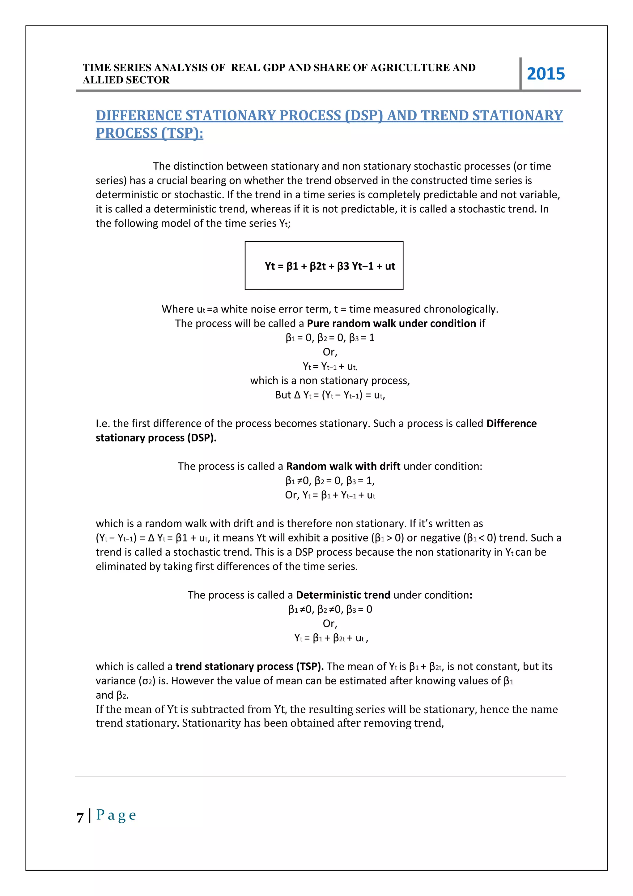
DIFFERENCE STATIONARY PROCESS (DSP) AND TREND STATIONARY
PROCESS (TSP):
The distinction between stationary and non stationary stochastic processes (or time
series) has a crucial bearing on whether the trend observed in the constructed time series is
deterministic or stochastic. If the trend in a time series is completely predictable and not variable,
it is called a deterministic trend, whereas if it is not predictable, it is called a stochastic trend. In
the following model of the time series Yt;
Yt = β + β t + β Yt− + ut
Where ut =a white noise error term, t = time measured chronologically.
The process will be called a Pure random walk under condition if
β1 = , β2 = , β3 = 1
Or,
Yt = Yt− + ut,
which is a non stationary process,
But Δ Yt = (Yt − Yt− ) = ut,
I.e. the first difference of the process becomes stationary. Such a process is called Difference
stationary process (DSP).
The process is called a Random walk with drift under condition:
β1 ≠ , β2 = , β3 = 1,
Or, Yt = β1 + Yt− + ut
which is a random walk with drift and is therefore non statio a . If it s itte as
(Yt − Yt− = Δ Yt = β + ut, it ea s Yt ill e hi it a positi e β1 > o egati e β1 < 0) trend. Such a
trend is called a stochastic trend. This is a DSP process because the non stationarity in Yt can be
eliminated by taking first differences of the time series.
The process is called a Deterministic trend under condition:
β1 ≠ , β2 ≠ , β3 = 0
Or,
Yt = β1 + β2t + ut ,
which is called a trend stationary process (TSP). The mean of Yt is β1 + β2t, is not constant, but its
a ia e σ2 is. Ho e e the alue of ea a e esti ated afte k o i g alues of β1
a d β2.
If the mean of Yt is subtracted from Yt, the resulting series will be stationary, hence the name
trend stationary. Stationarity has been obtained after removing trend,

ALLIED SECTOR 2015
8 | P a g e
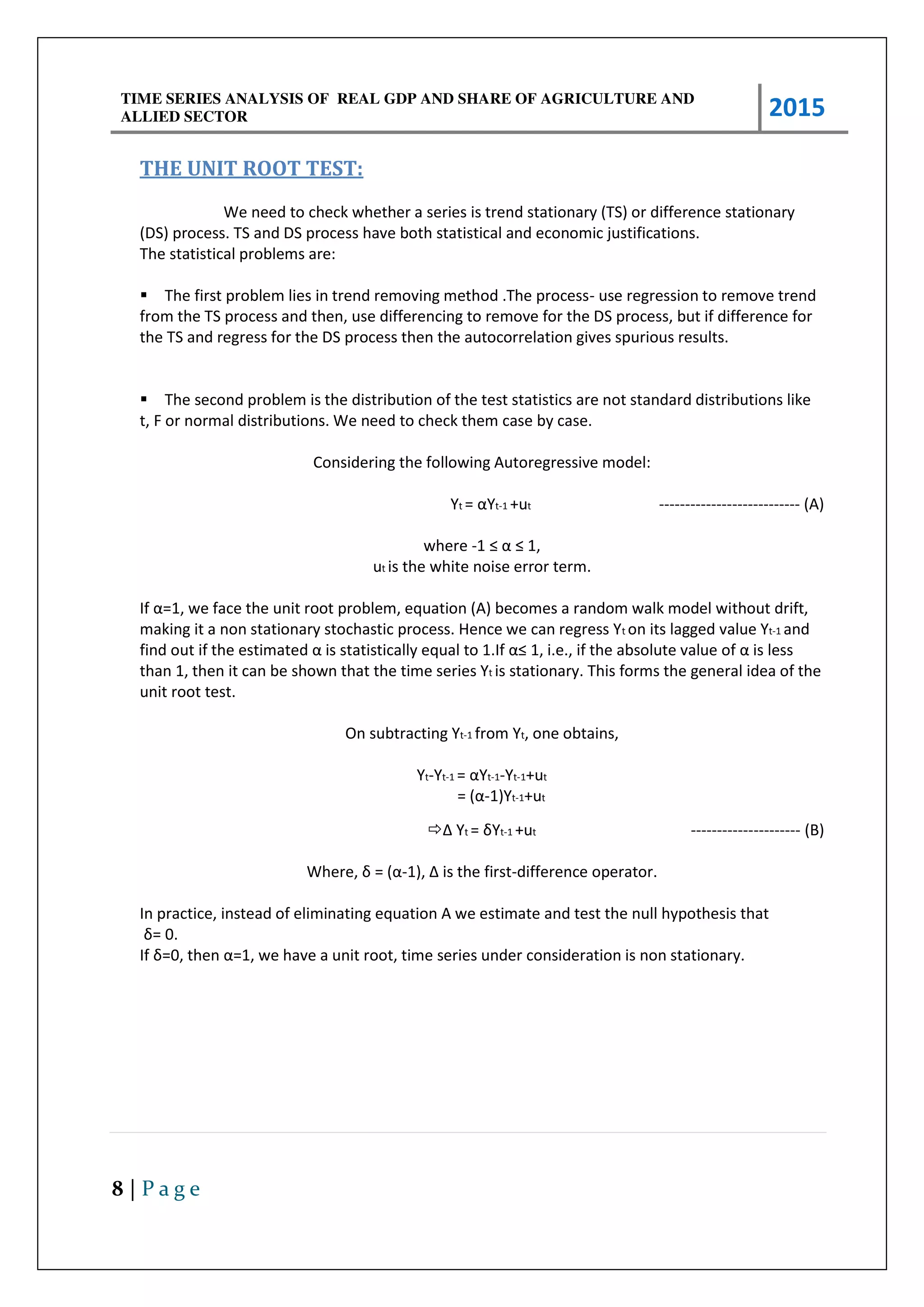
THE UNIT ROOT TEST:
We need to check whether a series is trend stationary (TS) or difference stationary
(DS) process. TS and DS process have both statistical and economic justifications.
The statistical problems are:
The first problem lies in trend removing method .The process- use regression to remove trend
from the TS process and then, use differencing to remove for the DS process, but if difference for
the TS and regress for the DS process then the autocorrelation gives spurious results.
The second problem is the distribution of the test statistics are not standard distributions like
t, F or normal distributions. We need to check them case by case.
Considering the following Autoregressive model:
Yt = αYt-1 +ut --------------------------- (A)
where - ≤ α ≤ ,
ut is the white noise error term.
If α= , e fa e the u it oot p o le , e uatio A e o es a a do alk odel ithout drift,
making it a non stationary stochastic process. Hence we can regress Yt on its lagged value Yt-1 and
fi d out if the esti ated α is statisti all e ual to .If α≤ , i.e., if the a solute alue of α is less
than 1, then it can be shown that the time series Yt is stationary. This forms the general idea of the
unit root test.
On subtracting Yt-1 from Yt, one obtains,
Yt-Yt-1 = αYt-1-Yt-1+ut
= α-1)Yt-1+ut
Δ Yt = Yt-1 +ut --------------------- (B)
Whe e, = α- , Δ is the fi st-difference operator.
In practice, instead of eliminating equation A we estimate and test the null hypothesis that
= .
If = , the α= , e ha e a u it oot, ti e se ies u de o side atio is o statio a .

ALLIED SECTOR 2015
9 | P a g e
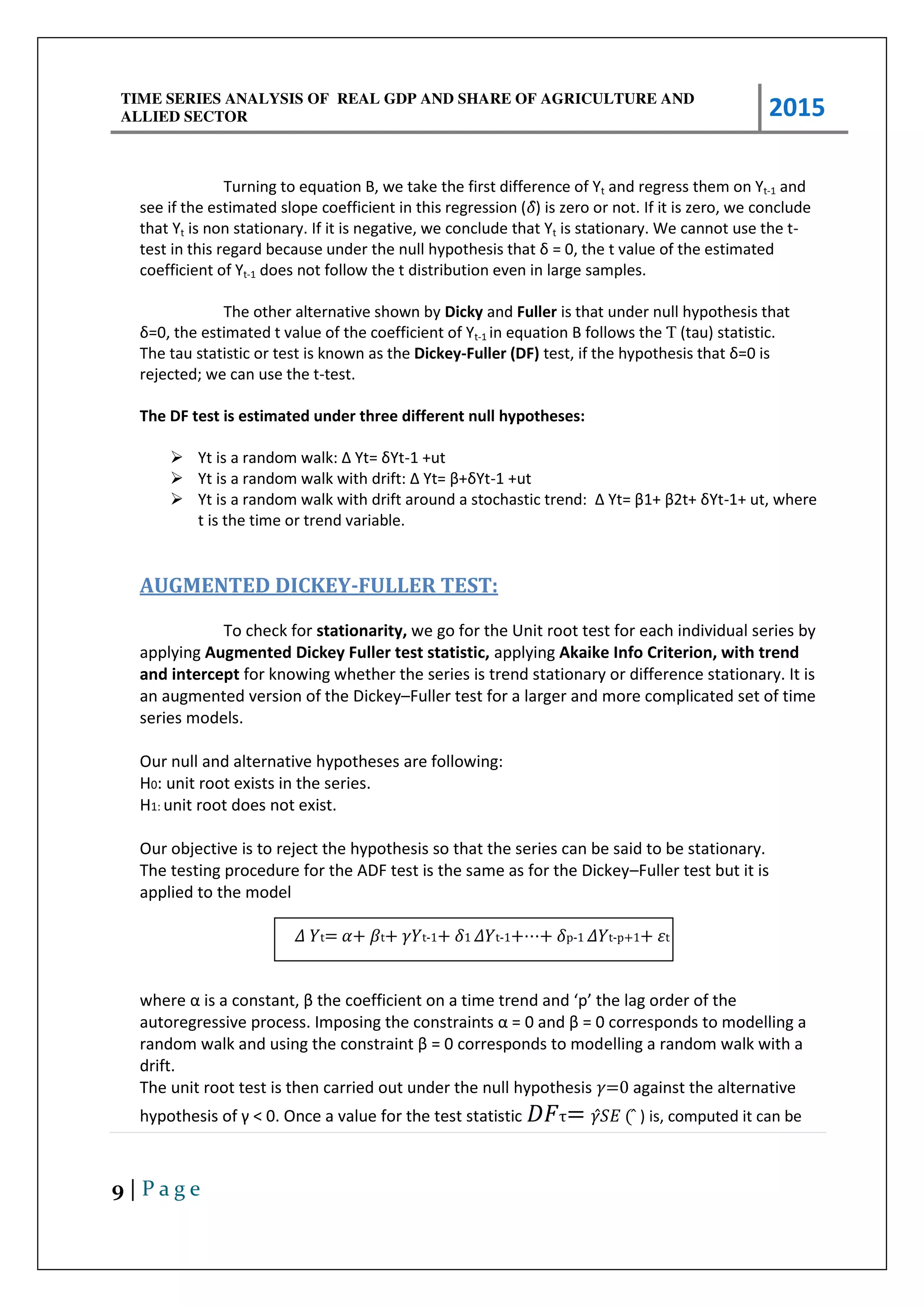
Turning to equation B, we take the first difference of Yt and regress them on Yt-1 and
see if the estimated slope coefficient in this regression (̂) is zero or not. If it is zero, we conclude
that Yt is non stationary. If it is negative, we conclude that Yt is stationary. We cannot use the t-
test i this ega d e ause u de the ull h pothesis that = , the t alue of the esti ated
coefficient of Yt-1 does not follow the t distribution even in large samples.
The other alternative shown by Dicky and Fuller is that under null hypothesis that
= , the esti ated t alue of the oeffi ie t of Yt-1 in equation B follows the Ƭ (tau) statistic.
The tau statistic or test is known as the Dickey-Fuller (DF) test, if the h pothesis that = is
rejected; we can use the t-test.
The DF test is estimated under three different null hypotheses:
 Yt is a a do alk: Δ Yt= Yt-1 +ut
 Yt is a a do alk ith d ift: Δ Yt= β+ Yt-1 +ut
 Yt is a a do alk ith d ift a ou d a sto hasti t e d: Δ Yt= β + β t+ Yt-1+ ut, where
t is the time or trend variable.
AUGMENTED DICKEY-FULLER TEST:
To check for stationarity, we go for the Unit root test for each individual series by
applying Augmented Dickey Fuller test statistic, applying Akaike Info Criterion, with trend
and intercept for knowing whether the series is trend stationary or difference stationary. It is
an augmented version of the Dickey–Fuller test for a larger and more complicated set of time
series models.
Our null and alternative hypotheses are following:
H0: unit root exists in the series.
H1: unit root does not exist.
Our objective is to reject the hypothesis so that the series can be said to be stationary.
The testing procedure for the ADF test is the same as for the Dickey–Fuller test but it is
applied to the model
� �t= + t+ �t-1+ ̂1 ��t-1+⋯+ ̂p-1 ��t-p+1+ �t
he e α is a o sta t, β the oeffi ie t o a ti e t e d a d p the lag o de of the
auto eg essi e p o ess. I posi g the o st ai ts α = a d β = o espo ds to odelli g a
a do alk a d usi g the o st ai t β = o espo ds to odelling a random walk with a
drift.
The unit root test is then carried out under the null hypothesis =0 against the alternative
h pothesis of < . O e a alue fo the test statisti τ= � ( ) is, computed it can be

ALLIED SECTOR 2015
10 | P a g e
compared to the relevant critical value for the Dickey–Fuller Test. If the test statistic is less (this
test is non symmetrical so we do not consider an absolute value) than the (larger negative) critical
value, then the null hypothesis of =0 is rejected and no unit root is present.
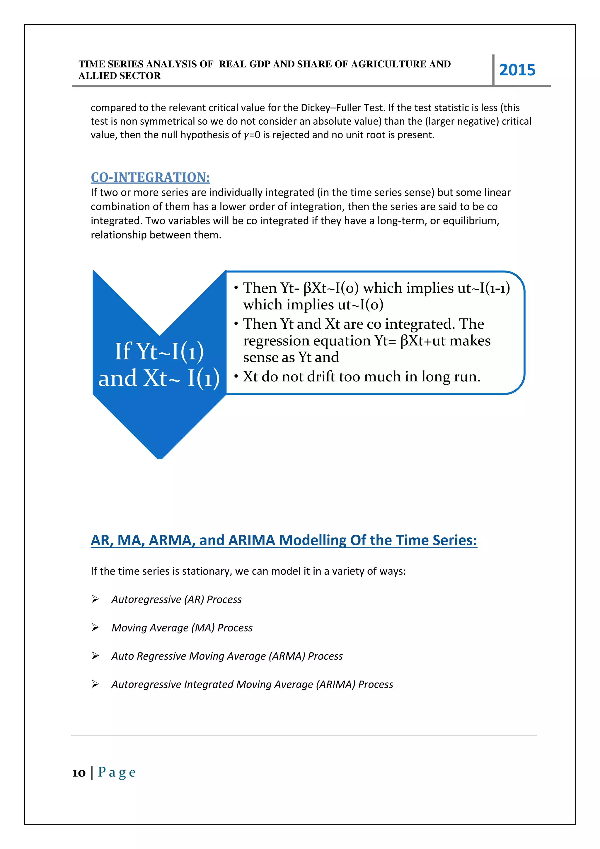
CO-INTEGRATION:
If two or more series are individually integrated (in the time series sense) but some linear
combination of them has a lower order of integration, then the series are said to be co
integrated. Two variables will be co integrated if they have a long-term, or equilibrium,
relationship between them.
AR, MA, ARMA, and ARIMA Modelling Of the Time Series:
If the time series is stationary, we can model it in a variety of ways:
Autoregressive (AR) Process
Moving Average (MA) Process
Auto Regressive Moving Average (ARMA) Process
Autoregressive Integrated Moving Average (ARIMA) Process
If Yt~I(1)
and Xt~ I(1)
• Then Yt- βXt~) which implies ut~) -1)
which implies ut~I(0)
• Then Yt and Xt are co integrated. The
regression equation Yt= βXt+ut makes
sense as Yt and
• Xt do not drift too much in long run.

ALLIED SECTOR 2015
11 | P a g e
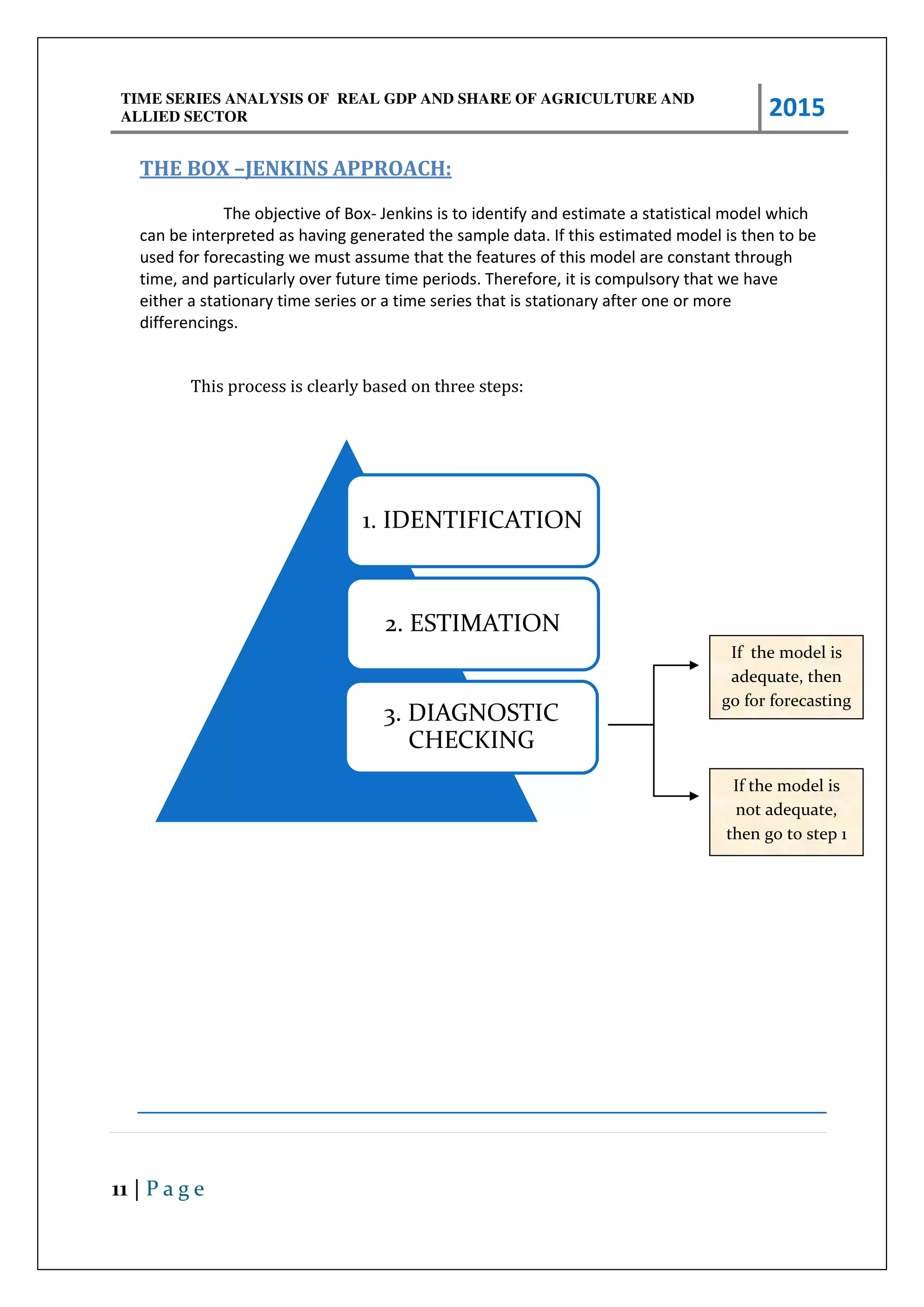
THE BOX –JENKINS APPROACH:
The objective of Box- Jenkins is to identify and estimate a statistical model which
can be interpreted as having generated the sample data. If this estimated model is then to be
used for forecasting we must assume that the features of this model are constant through
time, and particularly over future time periods. Therefore, it is compulsory that we have
either a stationary time series or a time series that is stationary after one or more
differencings.
This process is clearly based on three steps:
1. IDENTIFICATION
2. ESTIMATION
3. DIAGNOSTIC
CHECKING
If the model is
adequate, then
go for forecasting
If the model is
not adequate,
then go to step 1

ALLIED SECTOR 2015
12 | P a g e
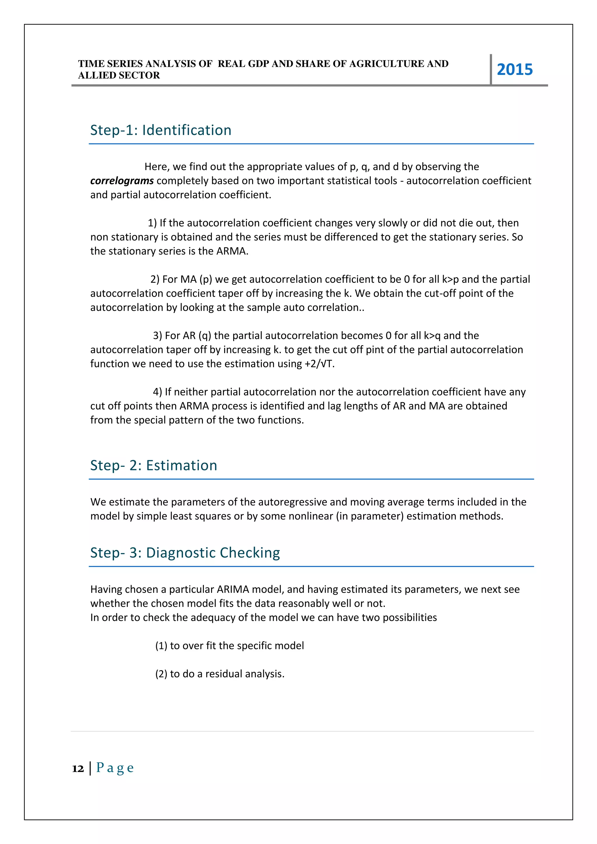
Step-1: Identification
Here, we find out the appropriate values of p, q, and d by observing the
correlograms completely based on two important statistical tools - autocorrelation coefficient
and partial autocorrelation coefficient.
1) If the autocorrelation coefficient changes very slowly or did not die out, then
non stationary is obtained and the series must be differenced to get the stationary series. So
the stationary series is the ARMA.
2) For MA (p) we get autocorrelation coefficient to be 0 for all k>p and the partial
autocorrelation coefficient taper off by increasing the k. We obtain the cut-off point of the
autocorrelation by looking at the sample auto correlation..
3) For AR (q) the partial autocorrelation becomes 0 for all k>q and the
autocorrelation taper off by increasing k. to get the cut off pint of the partial autocorrelation
function we need to use the estimatio usi g + /√T.
4) If neither partial autocorrelation nor the autocorrelation coefficient have any
cut off points then ARMA process is identified and lag lengths of AR and MA are obtained
from the special pattern of the two functions.
Step- 2: Estimation
We estimate the parameters of the autoregressive and moving average terms included in the
model by simple least squares or by some nonlinear (in parameter) estimation methods.
Step- 3: Diagnostic Checking
Having chosen a particular ARIMA model, and having estimated its parameters, we next see
whether the chosen model fits the data reasonably well or not.
In order to check the adequacy of the model we can have two possibilities
(1) to over fit the specific model
(2) to do a residual analysis.

ALLIED SECTOR 2015
13 | P a g e
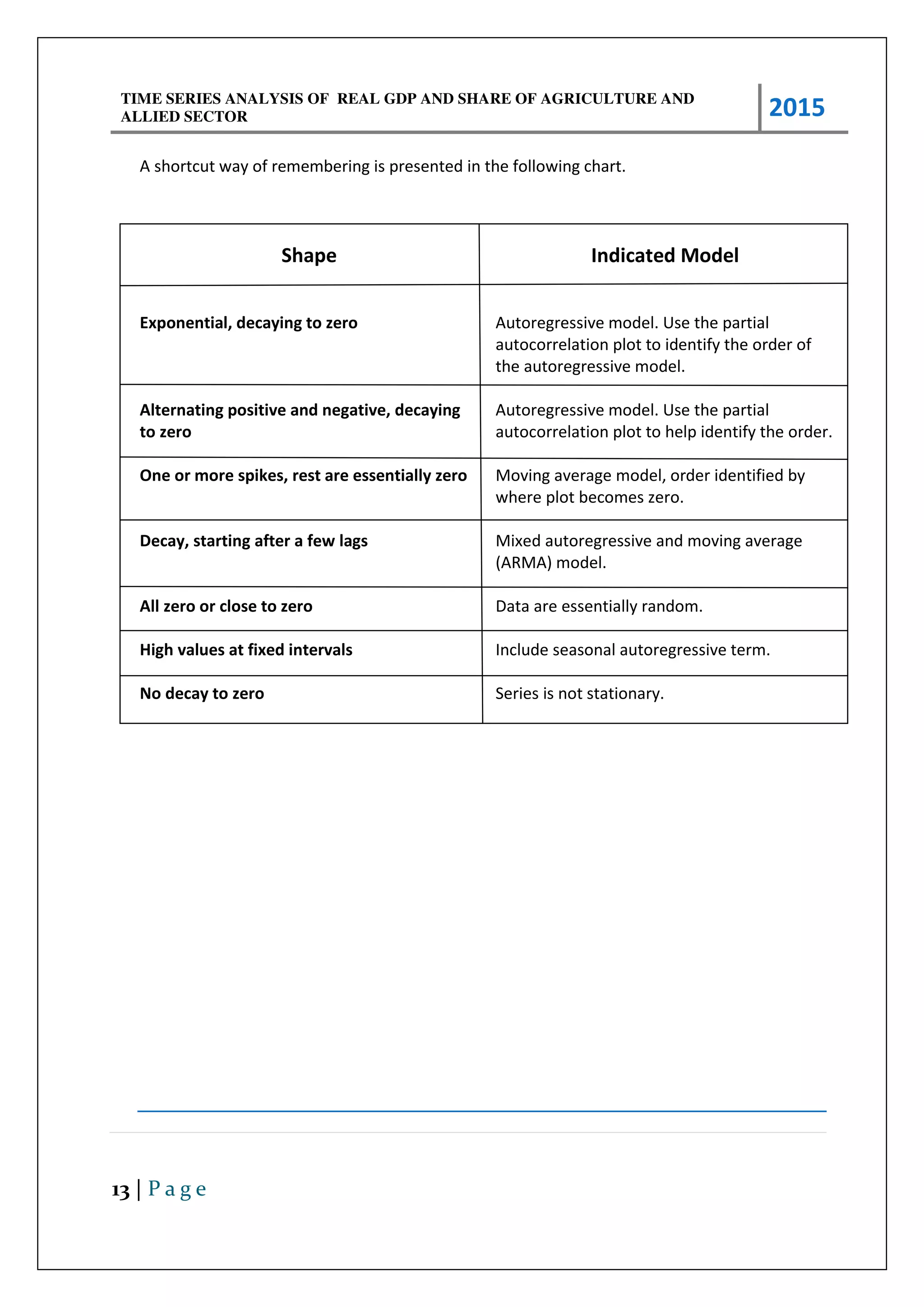
A shortcut way of remembering is presented in the following chart.
Shape Indicated Model
Exponential, decaying to zero Autoregressive model. Use the partial
autocorrelation plot to identify the order of
the autoregressive model.
Alternating positive and negative, decaying
to zero
Autoregressive model. Use the partial
autocorrelation plot to help identify the order.
One or more spikes, rest are essentially zero Moving average model, order identified by
where plot becomes zero.
Decay, starting after a few lags Mixed autoregressive and moving average
(ARMA) model.
All zero or close to zero Data are essentially random.
High values at fixed intervals Include seasonal autoregressive term.
No decay to zero Series is not stationary.

ALLIED SECTOR 2015
14 | P a g e
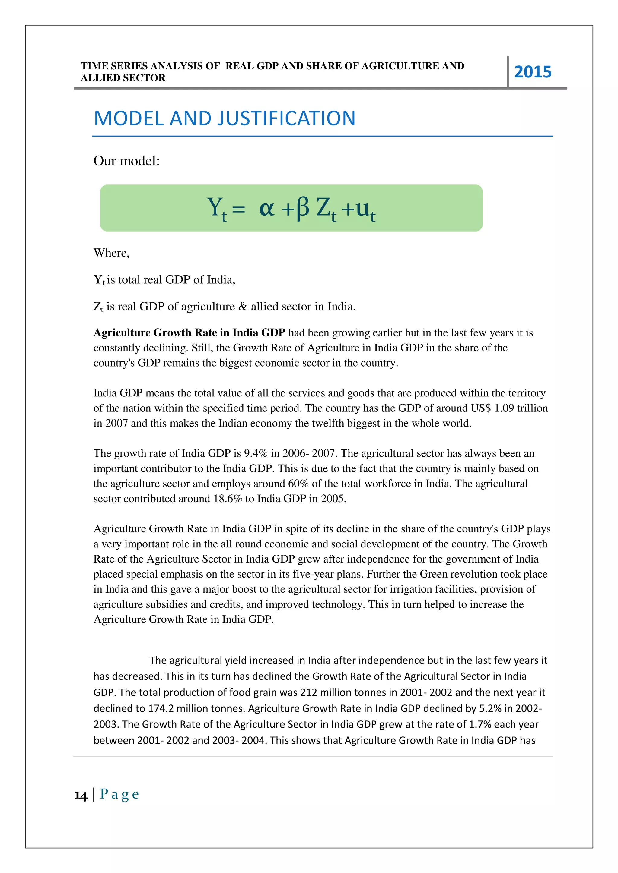
MODEL AND JUSTIFICATION
Our model:
Where,
Yt is total real GDP of India,
Zt is real GDP of agriculture & allied sector in India.
Agriculture Growth Rate in India GDP had been growing earlier but in the last few years it is
constantly declining. Still, the Growth Rate of Agriculture in India GDP in the share of the
country's GDP remains the biggest economic sector in the country.
India GDP means the total value of all the services and goods that are produced within the territory
of the nation within the specified time period. The country has the GDP of around US$ 1.09 trillion
in 2007 and this makes the Indian economy the twelfth biggest in the whole world.
The growth rate of India GDP is 9.4% in 2006- 2007. The agricultural sector has always been an
important contributor to the India GDP. This is due to the fact that the country is mainly based on
the agriculture sector and employs around 60% of the total workforce in India. The agricultural
sector contributed around 18.6% to India GDP in 2005.
Agriculture Growth Rate in India GDP in spite of its decline in the share of the country's GDP plays
a very important role in the all round economic and social development of the country. The Growth
Rate of the Agriculture Sector in India GDP grew after independence for the government of India
placed special emphasis on the sector in its five-year plans. Further the Green revolution took place
in India and this gave a major boost to the agricultural sector for irrigation facilities, provision of
agriculture subsidies and credits, and improved technology. This in turn helped to increase the
Agriculture Growth Rate in India GDP.
The agricultural yield increased in India after independence but in the last few years it
has decreased. This in its turn has declined the Growth Rate of the Agricultural Sector in India
GDP. The total production of food grain was 212 million tonnes in 2001- 2002 and the next year it
declined to 174.2 million tonnes. Agriculture Growth Rate in India GDP declined by 5.2% in 2002-
2003. The Growth Rate of the Agriculture Sector in India GDP grew at the rate of 1.7% each year
between 2001- 2002 and 2003- 2004. This shows that Agriculture Growth Rate in India GDP has
Yt = α +β Zt +ut

ALLIED SECTOR 2015
15 | P a g e
grown very slowly in the last few years.
Agriculture Growth Rate in India GDP has slowed down for the production in this sector has
reduced over the years. The agricultural sector has had low production due to a number of factors
such as illiteracy, insufficient FINANCE, and inadequate marketing of agricultural products. Further
the reasons for the decline in Agriculture Growth Rate in India GDP are that in the sector the
average size of the farms is very small which in turn has resulted in low productivity. Also the
Growth Rate of the Agricultural Sector in India GDP has declined due to the fact that the sector
has not adopted modern technology and agricultural practices. Agriculture Growth Rate in India
GDP has also decreased due to the fact that the sector has insufficient irrigation facilities. As a
result of this the farmers are dependent on rainfall, which is however very unpredictable.
Agriculture Growth Rate in India GDP has declined over the years. The Indian government must
take steps to boost the agricultural sector for this in its turn will lead to the growth of Agriculture
Growth Rate in India GDP.
"As per latest estimates released by Central Statistics Office (CSO) the share of agricultural
products/Agriculture and Allied Sectors in Gross Domestic Product (GDP) of the country was 51.9
per cent in 1950-51, which has now come down to 13.7 per cent in 2012-13 at 2004-05 prices,"
Minister of State for Agriculture
The Indian agriculture sector accounts for 18 per cent of India's gross domestic product (GDP) and employs
just a little less than 50 per cent of the country's workforce. This sector has made considerable progress in the
last few decades with its large resources of land, water and sunshine. India is presently the world's largest
producer of pulses and the second largest producer of rice and wheat.
The country is also the largest producer, consumer and exporter of spices and spice products in the world and
overall in farm and agriculture outputs, it is ranked second. From canned, dairy, processed, frozen food to
fisheries, meat, poultry, and food grains, the Indian agro industry has plenty of areas to choose for business.
The Department of Agriculture and Cooperation under the Ministry of Agriculture is the nodal organisation
responsible for the development of the agriculture sector in India. Under it, several other bodies such as the
National Dairy Development Board (NDDB) work for the development of the other allied agricultural sectors

ALLIED SECTOR 2015
16 | P a g e
ANALYSIS:-
METHODOLOGY :-
We have taken the time series data of the two variables (real gdp and agriculture and allied
se to s sha e i eal gdp o e a spa of ea s 9 -2014) and have tried to identify,
estimate and cross validate the time series processes using Box- Jenkins Method.
IDENTIFICATION & ESTIMATION
OF THE STOCHASTIC PROCESS
The first step of this method is to identify the stochastic process that each of
the time series variables follow. By observing the correlogram for every series we can
infer whether the series follows AR, MA or ARMA. To get the correlogram we kept the
maximum lag length 28 and the total sample observation was 60 (included data from
1954-55 to 2013-14). The correlograms for the series are given below.
The solid vertical line in the diagram (all correlogram diagrams) represents the
zero axis; observations above the line is positive values and below the line are negative
values.
We have used the Box- Jenkins approach to throw light on the empirical analysis of
our data. According to this approach we need to follow three steps to find the long run
relationship between dependent variable and all independent variables. In our paper we have one
dependent variable i.e. growth f TOTAL REAL GDP and one independent variables i.e. GDP of
agriculture & allied sector.

ALLIED SECTOR 2015
17 | P a g e
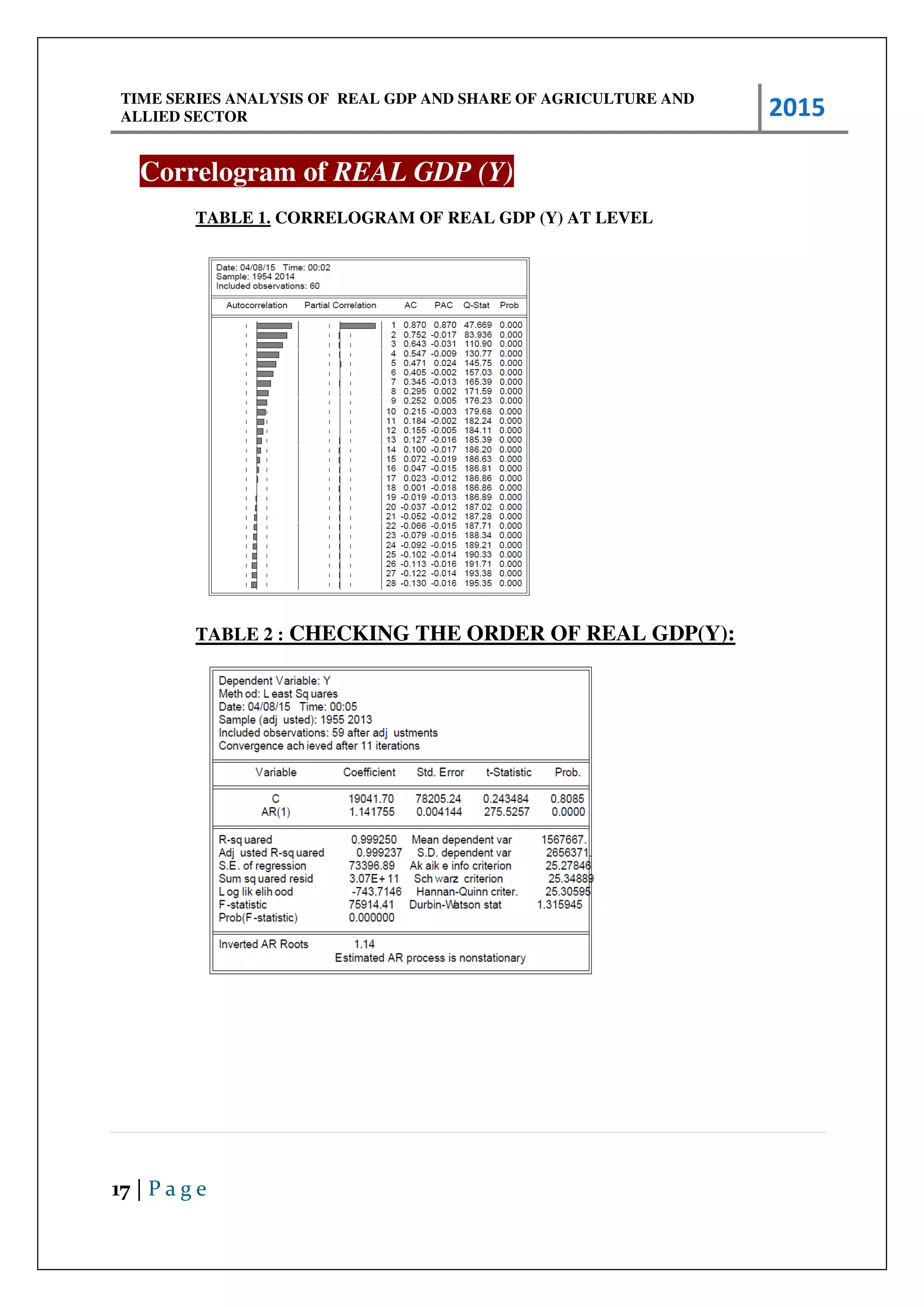
Correlogram of REAL GDP (Y)
TABLE 1. CORRELOGRAM OF REAL GDP (Y) AT LEVEL
TABLE 2 : CHECKING THE ORDER OF REAL GDP(Y):

ALLIED SECTOR 2015
18 | P a g e
From the graphical representation of Y, we can identify that Y follows auto regressive
process of order 1,AR(1). The partial auto-correlation function is
positive and significant only for K=1 and beyond that it falls below the critical region.
Moreover, the auto-correlation function is tapering as K is increasing.
We now estimate this AR(1) process. To have a stationary AR(1) process we need to
have the inverted AR root, |p|<1. But, here, we have obtained that |p| >1.
This implies that for every unit change in Yt-1 there is a greater change in Yt. This
further implies that the series will continue to be non-stationary over time. Though value of the t-
statistics of the AR (1) process is statistically significant, having a non-stationary series is not
desirable.
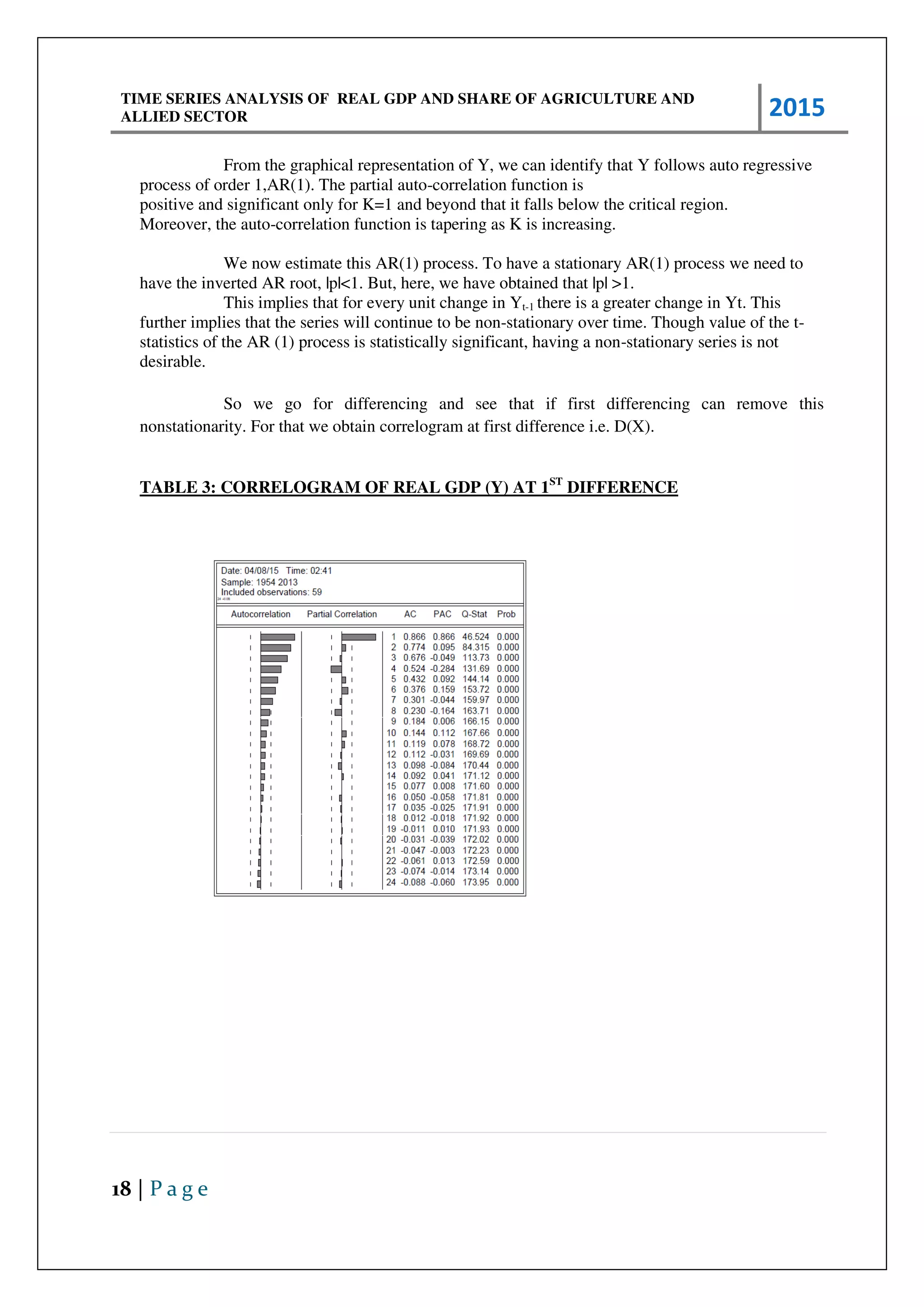
So we go for differencing and see that if first differencing can remove this
nonstationarity. For that we obtain correlogram at first difference i.e. D(X).
TABLE 3: CORRELOGRAM OF REAL GDP (Y) AT 1ST
DIFFERENCE

ALLIED SECTOR 2015
19 | P a g e
TABLE 4: CHECKING THE ORDER OF REAL GDP(Y) AT FIRST
DIFFERENCE:
Dependent Variable: D(Y)
Method: Least Squares
Date: 04/10/15 Time: 23:21
Sample (adjusted): 1956 2013
Included observations: 58 after adjustments
Convergence achieved after 8 iterations
Variable Coefficient Std. Error t-Statistic Prob.
C -111371.5 185301.8 -0.601027 0.5502
AR(1) 1.080524 0.035968 30.04138 0.0000
R-squared 0.941574 Mean dependent var 195581.1
Adjusted R-squared 0.940531 S.D. dependent var 339592.6
S.E. of regression 82813.87 Akaike info criterion 25.52045
Sum squared resid 3.84E+11 Schwarz criterion 25.59150
Log likelihood -738.0931 Hannan-Quinn criter. 25.54813
F-statistic 902.4844 Durbin-Watson stat 2.111862
Prob(F-statistic) 0.000000
Inverted AR Roots 1.08
Estimated AR process is nonstationary
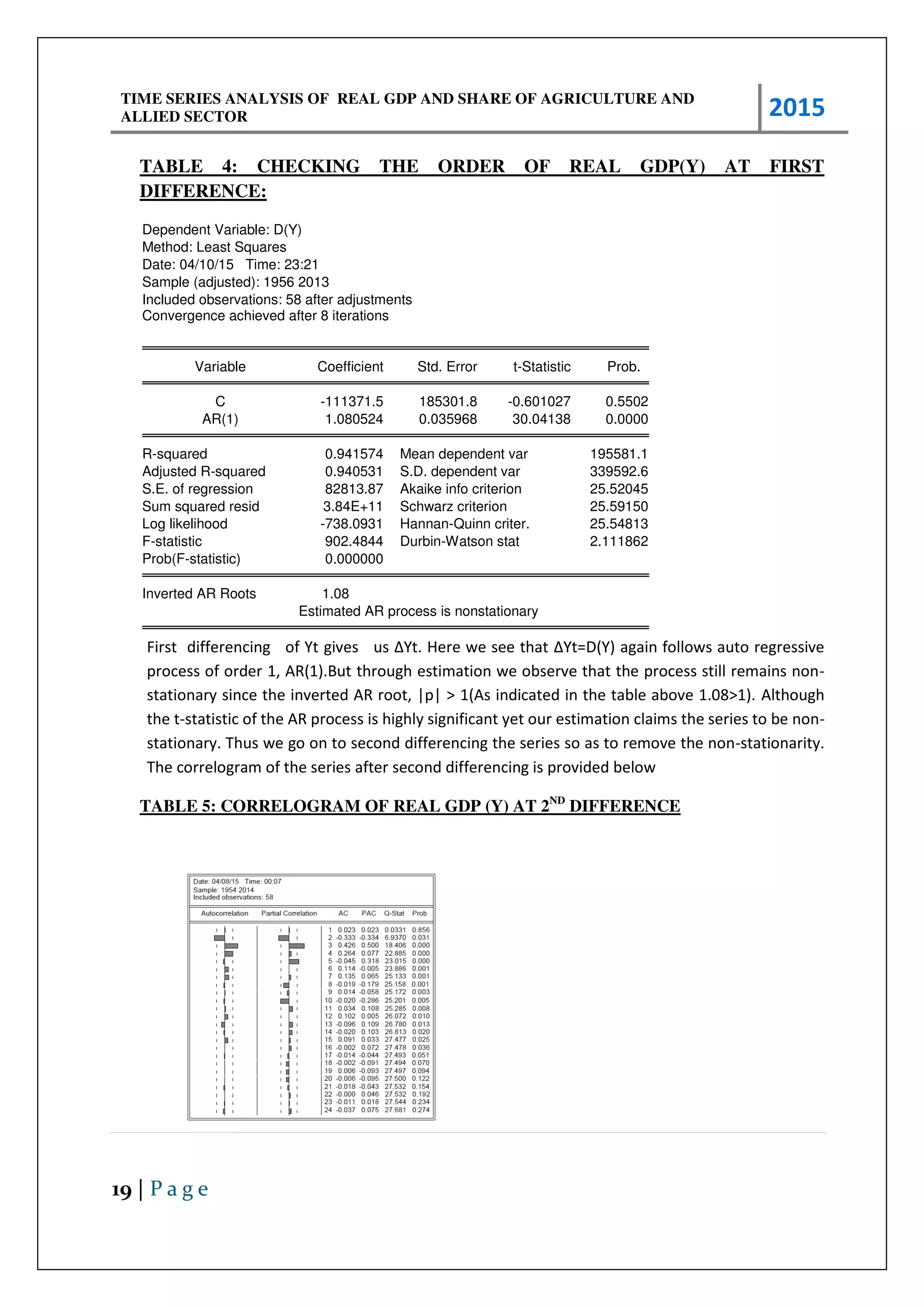
First differencing of Yt gi es us ΔYt. He e e see that ∆Yt=D(Y) again follows auto regressive
process of order 1, AR(1).But through estimation we observe that the process still remains non-
stationary since the inverted AR root, |p| > 1(As indicated in the table above 1.08>1). Although
the t-statistic of the AR process is highly significant yet our estimation claims the series to be non-
stationary. Thus we go on to second differencing the series so as to remove the non-stationarity.
The correlogram of the series after second differencing is provided below
TABLE 5: CORRELOGRAM OF REAL GDP (Y) AT 2ND
DIFFERENCE

ALLIED SECTOR 2015
20 | P a g e
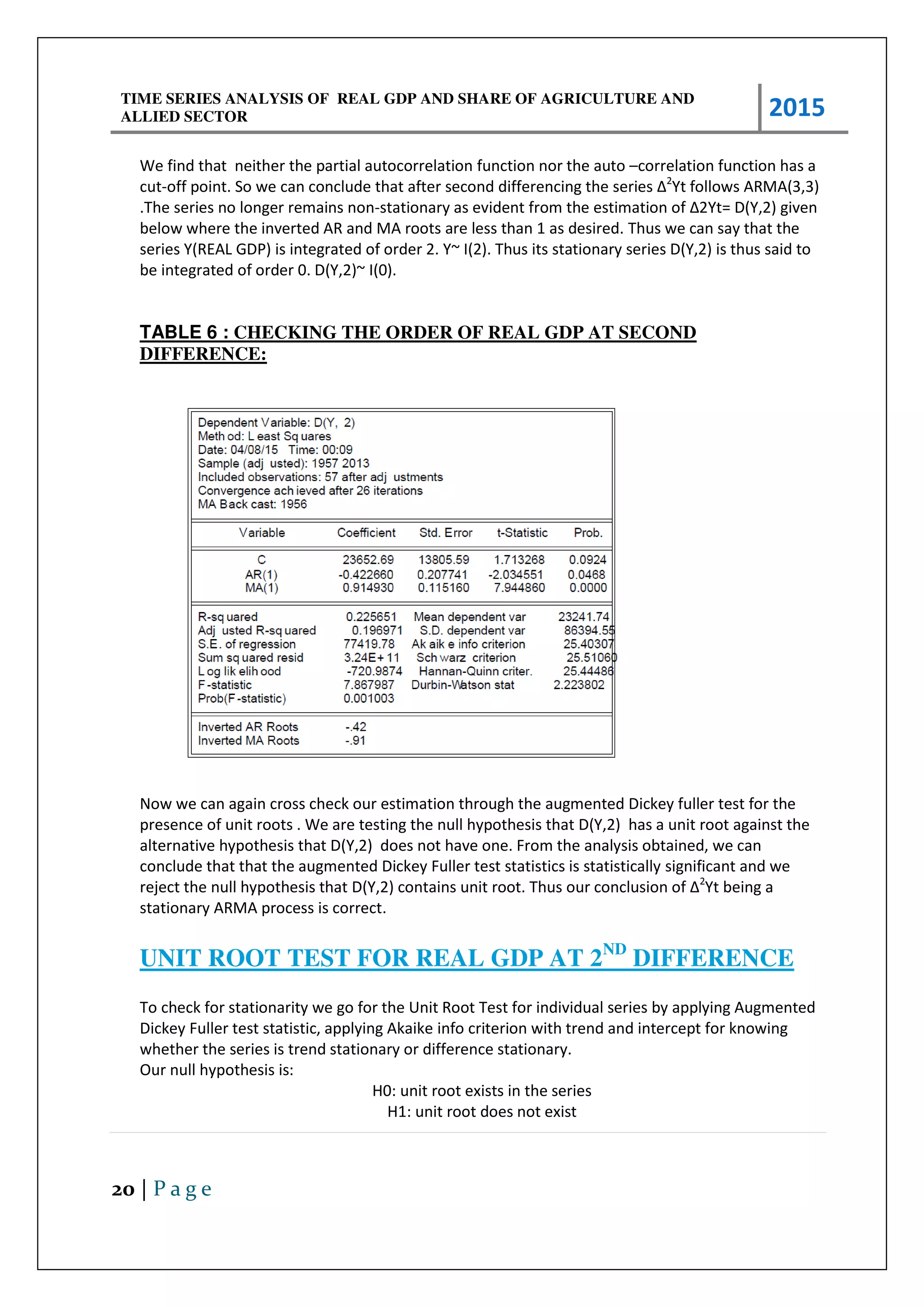
We find that neither the partial autocorrelation function nor the auto –correlation function has a
cut-off point. So we can conclude that after second differencing the se ies Δ2
Yt follows ARMA(3,3)
.The series no longer remains non-stationary as evident from the estimation of ∆ Yt= D(Y,2) given
below where the inverted AR and MA roots are less than 1 as desired. Thus we can say that the
series Y(REAL GDP) is integrated of order 2. Y~ I(2). Thus its stationary series D(Y,2) is thus said to
be integrated of order 0. D(Y,2)~ I(0).
TABLE 6 : CHECKING THE ORDER OF REAL GDP AT SECOND
DIFFERENCE:
Now we can again cross check our estimation through the augmented Dickey fuller test for the
presence of unit roots . We are testing the null hypothesis that D(Y,2) has a unit root against the
alternative hypothesis that D(Y,2) does not have one. From the analysis obtained, we can
conclude that that the augmented Dickey Fuller test statistics is statistically significant and we
reject the null hypothesis that D(Y,2) o tai s u it oot. Thus ou o lusio of Δ2
Yt being a
stationary ARMA process is correct.
UNIT ROOT TEST FOR REAL GDP AT 2ND
DIFFERENCE
To check for stationarity we go for the Unit Root Test for individual series by applying Augmented
Dickey Fuller test statistic, applying Akaike info criterion with trend and intercept for knowing
whether the series is trend stationary or difference stationary.
Our null hypothesis is:
H0: unit root exists in the series
H1: unit root does not exist

ALLIED SECTOR 2015
21 | P a g e
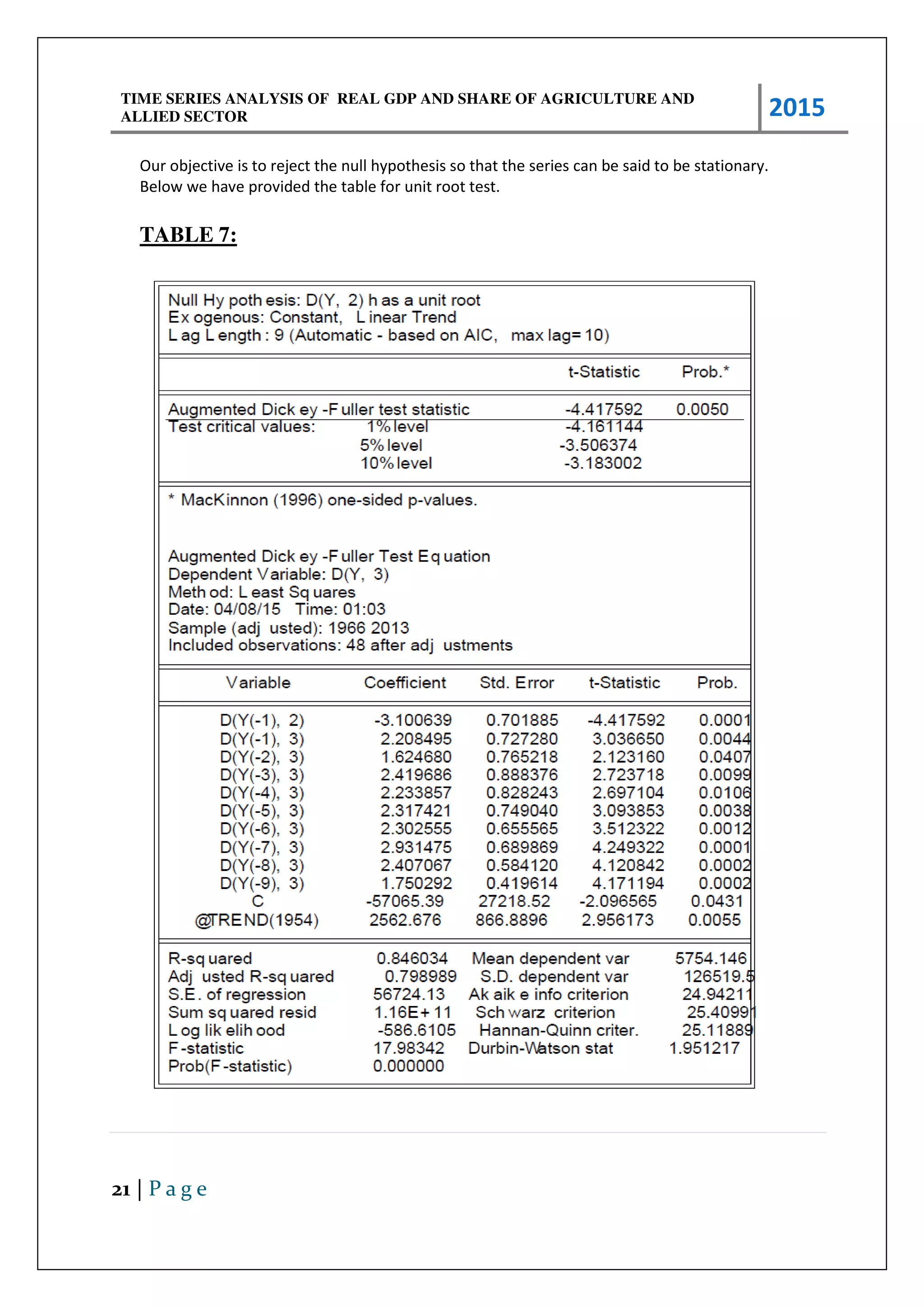
Our objective is to reject the null hypothesis so that the series can be said to be stationary.
Below we have provided the table for unit root test.
TABLE 7:

ALLIED SECTOR 2015
22 | P a g e
From the tabular result:
The computed value of t-statistic = -4.417592
Critical value of Augmented Dickey Fuller test statistic
at level 1% = -4.161144
at level 5% = -3.506374
at level 10% = -3.183002
Clearly, 4.417592 >4.161144, 4.417592 >3.506374 and 4.417592 >3.183002.
So, we have sufficient evidence to reject the null hypothesis at 10%, 5%, and even 1%. Hence we
conclude that the unit root does not exist and the series is stationary.
From here we can imply:
D(y, 2) ~ I(0)
Y ~ I(2)
Thus real GDP follows I (2).
After the entire process of identification and estimation we move on to the third stage of the
Box-Jenkins Method namely cross validation or diagnostic checking.
CROSS VALIDATION OR DIAGNOSTIC
CHECKING
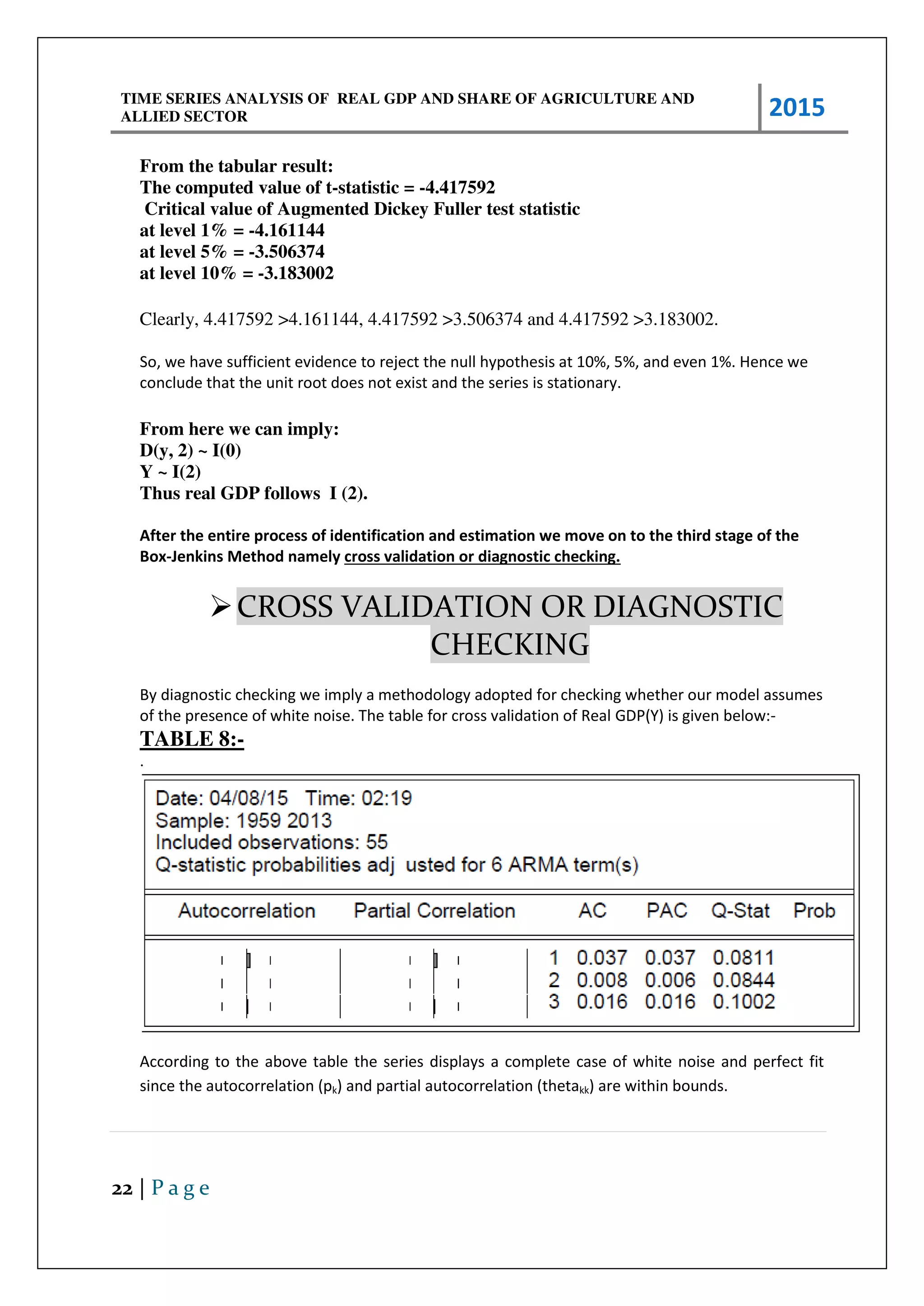
By diagnostic checking we imply a methodology adopted for checking whether our model assumes
of the presence of white noise. The table for cross validation of Real GDP(Y) is given below:-
TABLE 8:-
.
According to the above table the series displays a complete case of white noise and perfect fit
since the autocorrelation (pk) and partial autocorrelation (thetakk) are within bounds.

ALLIED SECTOR 2015
23 | P a g e
CORRELOGRAM OF SHARE OF AGRICULTURE AND ALLIED
SECTOR TO REAL GDP (IN REAL TERMS) BASE YEAR 2004-
05.(DENOTED BY Z)
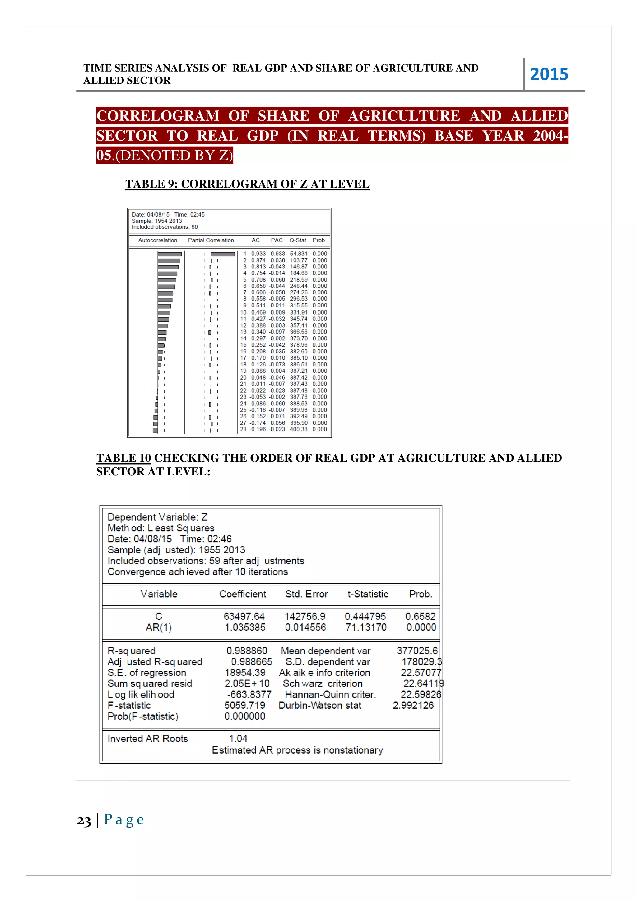
TABLE 9: CORRELOGRAM OF Z AT LEVEL
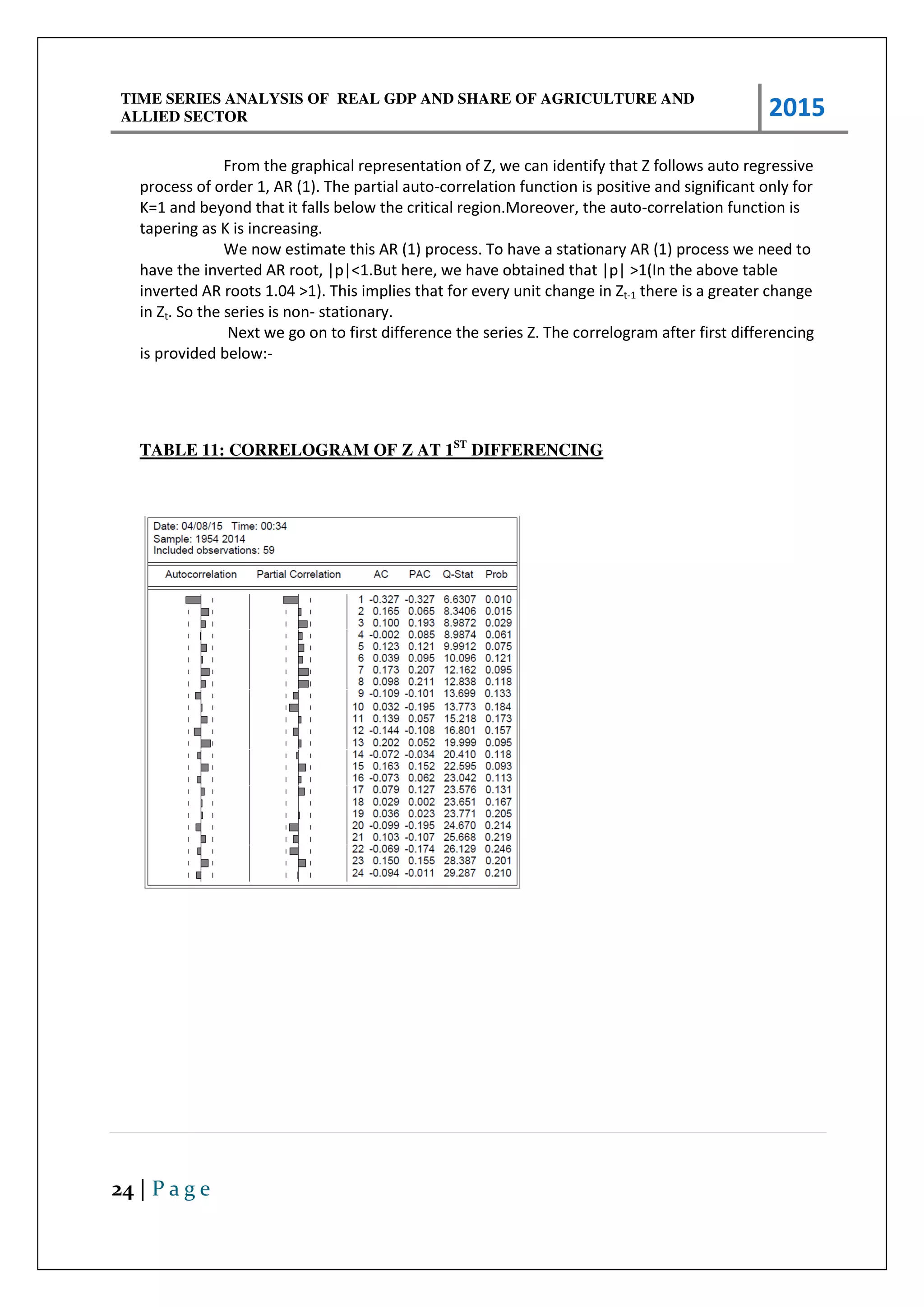
TABLE 10 CHECKING THE ORDER OF REAL GDP AT AGRICULTURE AND ALLIED
SECTOR AT LEVEL:

ALLIED SECTOR 2015
24 | P a g e
From the graphical representation of Z, we can identify that Z follows auto regressive
process of order 1, AR (1). The partial auto-correlation function is positive and significant only for
K=1 and beyond that it falls below the critical region.Moreover, the auto-correlation function is
tapering as K is increasing.
We now estimate this AR (1) process. To have a stationary AR (1) process we need to
have the inverted AR root, |p|<1.But here, we have obtained that |p| >1(In the above table
inverted AR roots 1.04 >1). This implies that for every unit change in Zt-1 there is a greater change
in Zt. So the series is non- stationary.
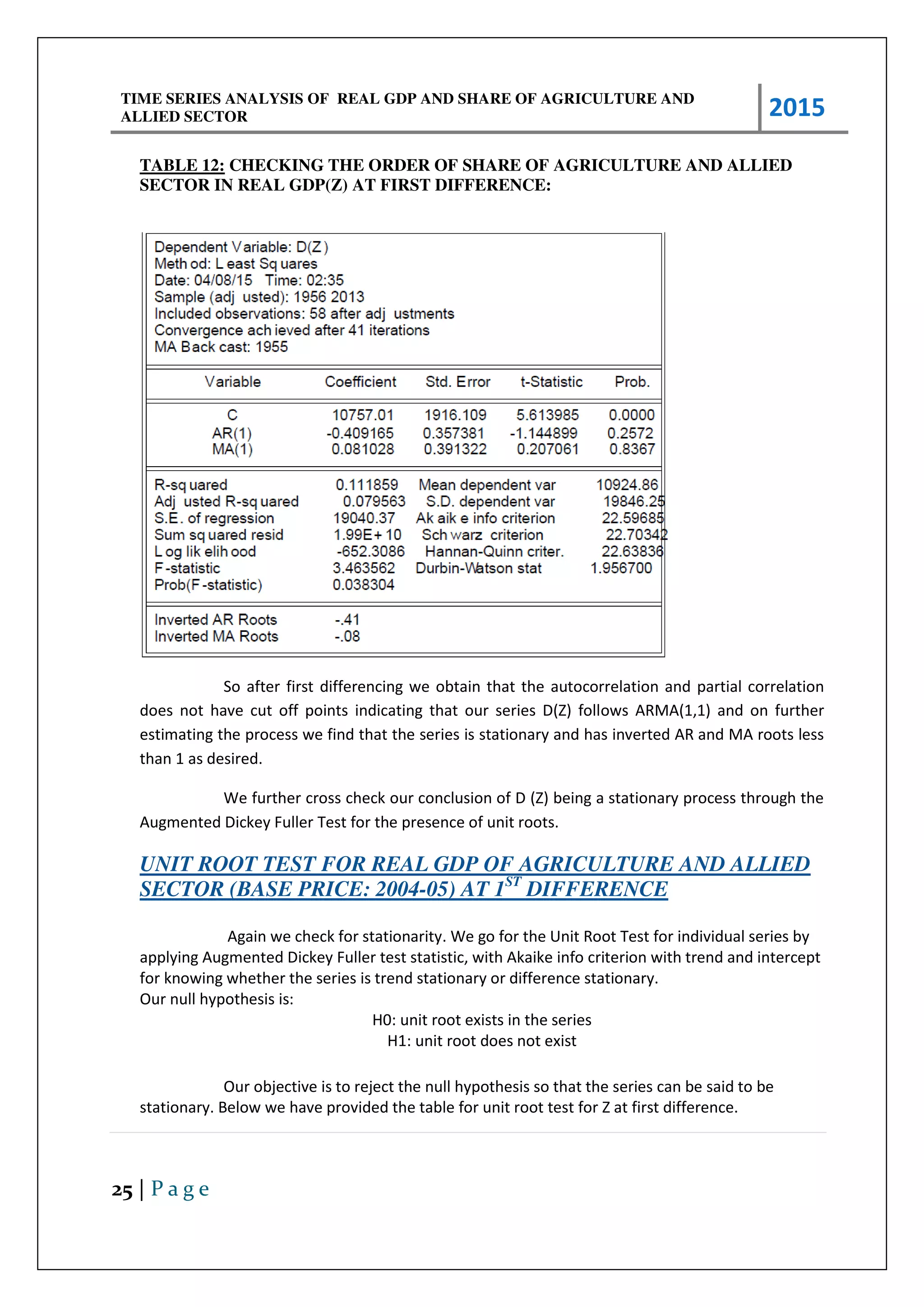
Next we go on to first difference the series Z. The correlogram after first differencing
is provided below:-
TABLE 11: CORRELOGRAM OF Z AT 1ST
DIFFERENCING

ALLIED SECTOR 2015
25 | P a g e
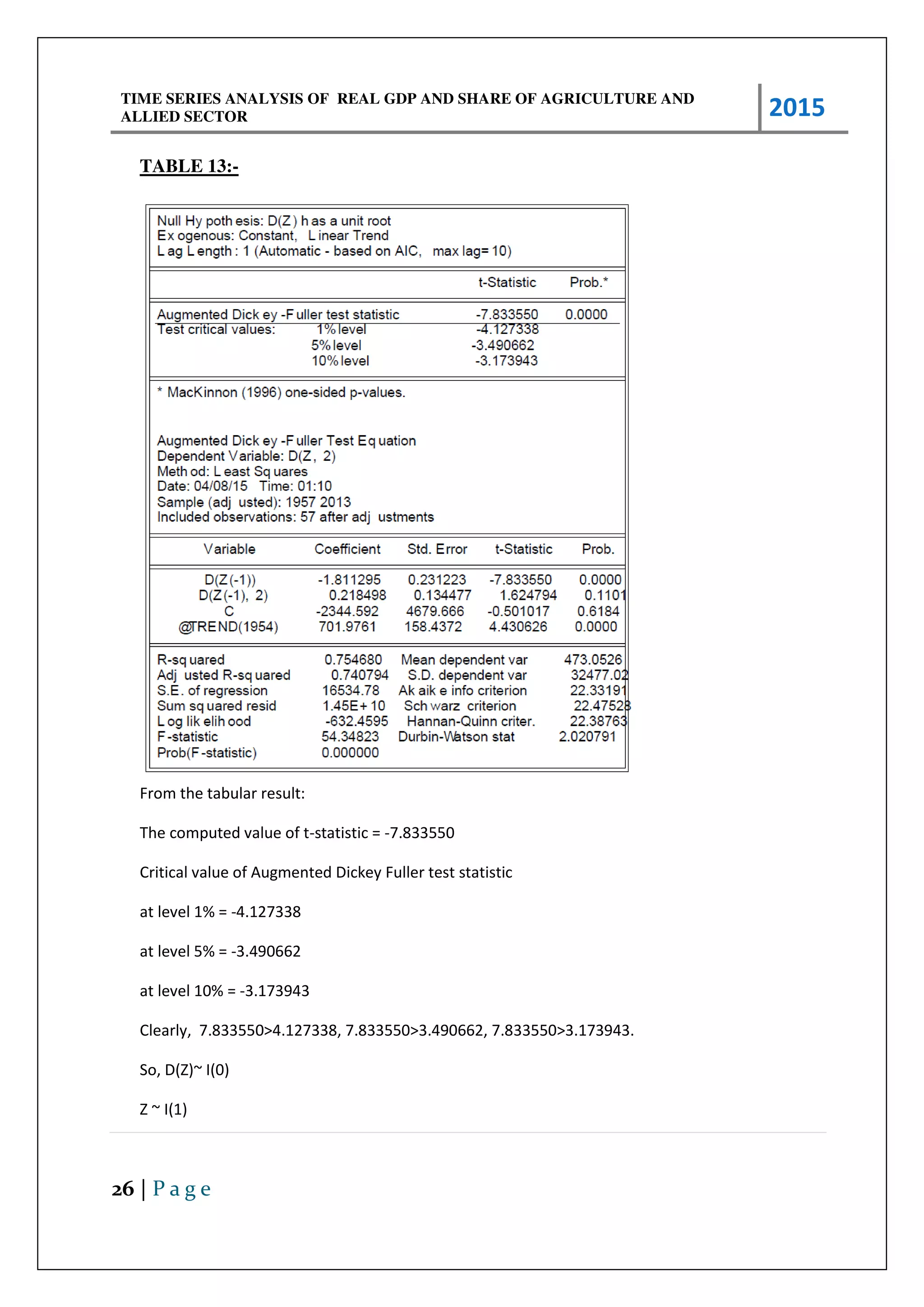
TABLE 12: CHECKING THE ORDER OF SHARE OF AGRICULTURE AND ALLIED
SECTOR IN REAL GDP(Z) AT FIRST DIFFERENCE:
So after first differencing we obtain that the autocorrelation and partial correlation
does not have cut off points indicating that our series D(Z) follows ARMA(1,1) and on further
estimating the process we find that the series is stationary and has inverted AR and MA roots less
than 1 as desired.
We further cross check our conclusion of D (Z) being a stationary process through the
Augmented Dickey Fuller Test for the presence of unit roots.
UNIT ROOT TEST FOR REAL GDP OF AGRICULTURE AND ALLIED
SECTOR (BASE PRICE: 2004-05) AT 1ST
DIFFERENCE
Again we check for stationarity. We go for the Unit Root Test for individual series by
applying Augmented Dickey Fuller test statistic, with Akaike info criterion with trend and intercept
for knowing whether the series is trend stationary or difference stationary.
Our null hypothesis is:
H0: unit root exists in the series
H1: unit root does not exist
Our objective is to reject the null hypothesis so that the series can be said to be
stationary. Below we have provided the table for unit root test for Z at first difference.

ALLIED SECTOR 2015
26 | P a g e
TABLE 13:-
From the tabular result:
The computed value of t-statistic = -7.833550
Critical value of Augmented Dickey Fuller test statistic
at level 1% = -4.127338
at level 5% = -3.490662
at level 10% = -3.173943
Clearly, 7.833550>4.127338, 7.833550>3.490662, 7.833550>3.173943.
So, D(Z)~ I(0)
Z ~ I(1)

ALLIED SECTOR 2015
27 | P a g e
Hence real GDP of agriculture and allied sector follows I(1).
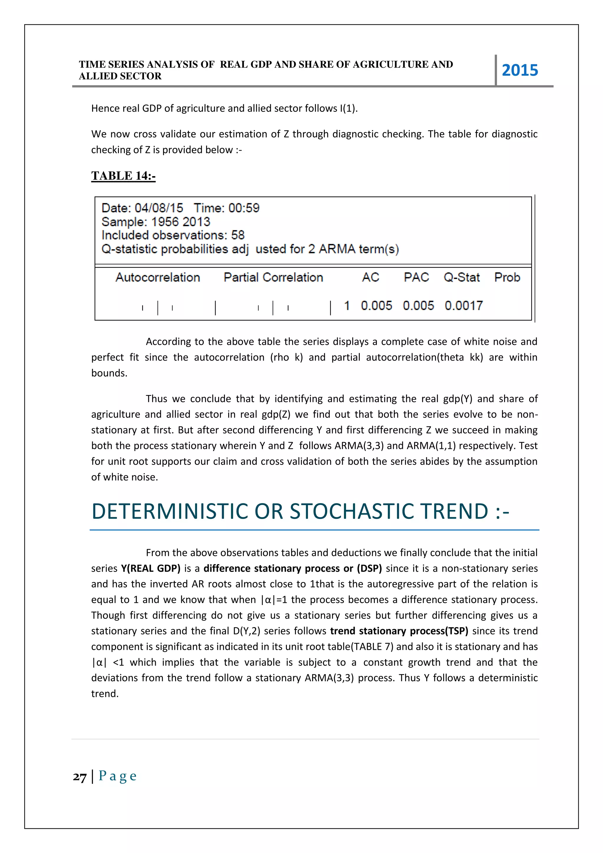
We now cross validate our estimation of Z through diagnostic checking. The table for diagnostic
checking of Z is provided below :-
TABLE 14:-
According to the above table the series displays a complete case of white noise and
perfect fit since the autocorrelation (rho k) and partial autocorrelation(theta kk) are within
bounds.
Thus we conclude that by identifying and estimating the real gdp(Y) and share of
agriculture and allied sector in real gdp(Z) we find out that both the series evolve to be non-
stationary at first. But after second differencing Y and first differencing Z we succeed in making
both the process stationary wherein Y and Z follows ARMA(3,3) and ARMA(1,1) respectively. Test
for unit root supports our claim and cross validation of both the series abides by the assumption
of white noise.
DETERMINISTIC OR STOCHASTIC TREND :-
From the above observations tables and deductions we finally conclude that the initial
series Y(REAL GDP) is a difference stationary process or (DSP) since it is a non-stationary series
and has the inverted AR roots almost close to 1that is the autoregressive part of the relation is
equal to 1 and we know that he |α|= the p o ess e o es a diffe e e statio a p o ess.
Though first differencing do not give us a stationary series but further differencing gives us a
stationary series and the final D(Y,2) series follows trend stationary process(TSP) since its trend
component is significant as indicated in its unit root table(TABLE 7) and also it is stationary and has
|α| < hi h i plies that the a ia le is su je t to a constant growth trend and that the
deviations from the trend follow a stationary ARMA(3,3) process. Thus Y follows a deterministic
trend.

ALLIED SECTOR 2015
28 | P a g e
Similarly Z(SHARE OF AGRICULTURE AND ALLIED SECTORS IN REAL GDP) is a
difference stationary process(DSP) since it is non-stationary and has inverted AR roots greater
than 1 or almost close to 1 for which it reduces to a difference stationary process. Further
differencing of Z gives us a stationary series D(Z) which on the other hand follows Trend
Stationary Process(TSP) of ARMA(1,1) e ause he e |α| <1 and also its trend component is
significant as indicated in the unit root test for D(Z)(TABLE 12). Thus we can say that Z follows a
deterministic trend.
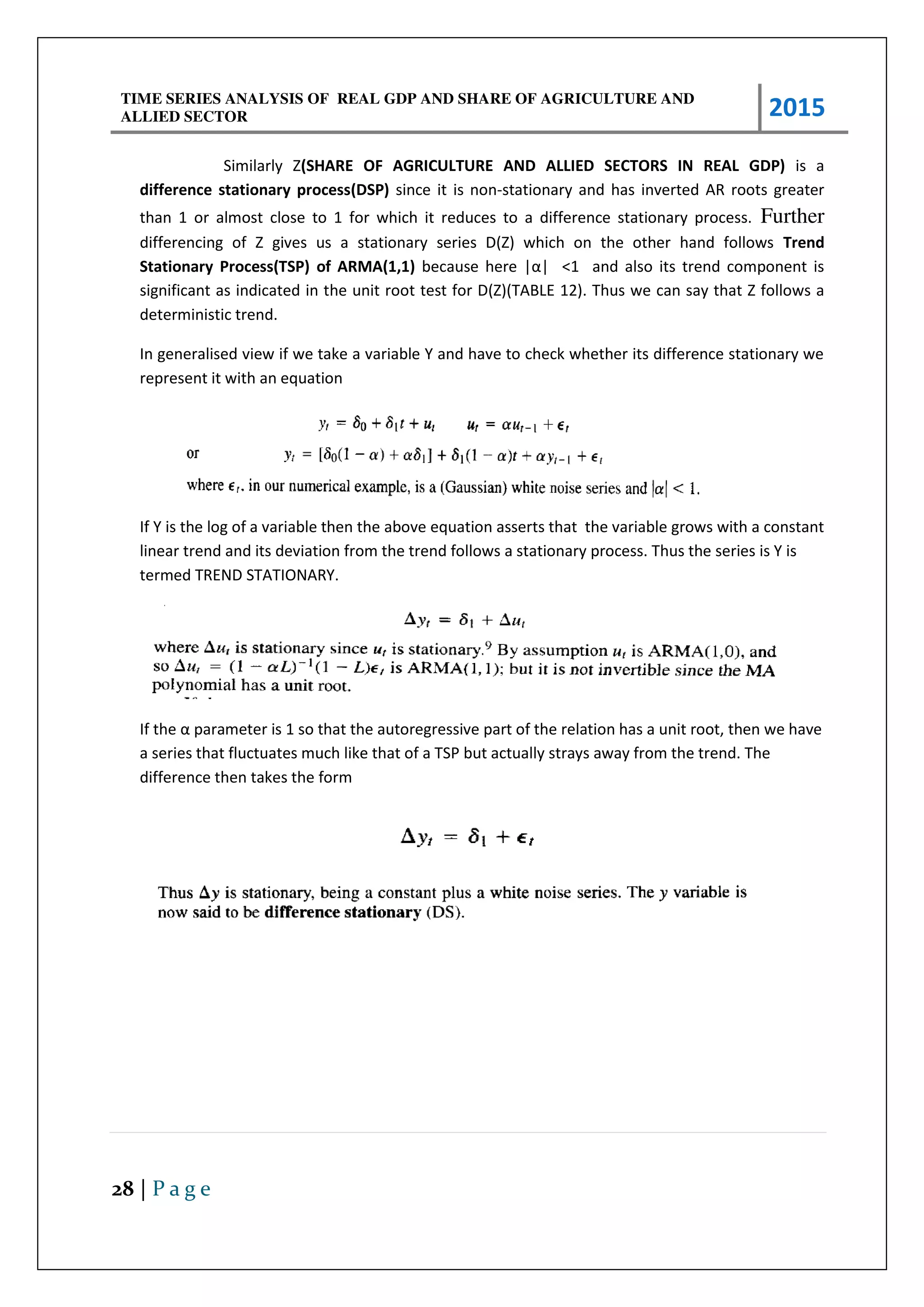
In generalised view if we take a variable Y and have to check whether its difference stationary we
represent it with an equation
If Y is the log of a variable then the above equation asserts that the variable grows with a constant
linear trend and its deviation from the trend follows a stationary process. Thus the series is Y is
termed TREND STATIONARY.
If the α pa a ete is so that the auto eg essi e pa t of the elatio has a u it oot, the e ha e
a series that fluctuates much like that of a TSP but actually strays away from the trend. The
difference then takes the form

ALLIED SECTOR 2015
29 | P a g e
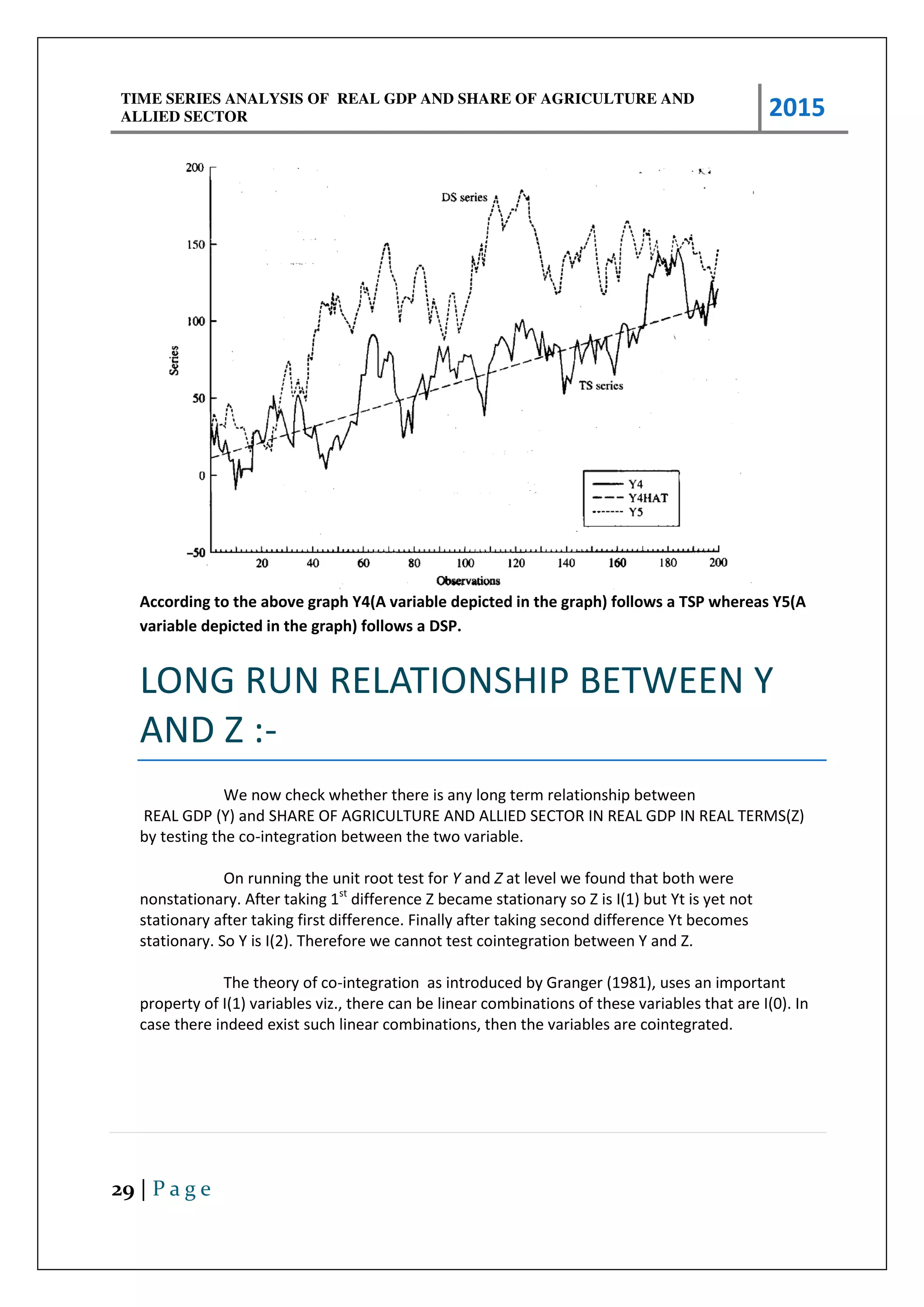
According to the above graph Y4(A variable depicted in the graph) follows a TSP whereas Y5(A
variable depicted in the graph) follows a DSP.
LONG RUN RELATIONSHIP BETWEEN Y
AND Z :-
We now check whether there is any long term relationship between
REAL GDP (Y) and SHARE OF AGRICULTURE AND ALLIED SECTOR IN REAL GDP IN REAL TERMS(Z)
by testing the co-integration between the two variable.
On running the unit root test for Y and Z at level we found that both were
nonstationary. After taking 1st
difference Z became stationary so Z is I(1) but Yt is yet not
stationary after taking first difference. Finally after taking second difference Yt becomes
stationary. So Y is I(2). Therefore we cannot test cointegration between Y and Z.
The theory of co-integration as introduced by Granger (1981), uses an important
property of I(1) variables viz., there can be linear combinations of these variables that are I(0). In
case there indeed exist such linear combinations, then the variables are cointegrated.

ALLIED SECTOR 2015
30 | P a g e
But since here our variables are not cointegrated thus there does not exist any long
term relationship between Y and Z as per the data of our model.( TABLE 7 FOR Y AND TABLE 12
FOR Z)
Since we cannot compute any co-integration between Y and Z thus we do not need to
find out the residual variable and compute its unit root since even if it suffices for the assumption
of white noise it is of no help in computing co-integration between Y and Z.
Y~ I(2)
Z ~ I(1)
E(Error term) satisfy the assumption of white noise so E~I(0)
Still we cannot cointegrate Y and Z.
So we can conclude that from our previous knowledge of econometric analysis
compelled us to always compute a regression between two given variables but further
knowledge on time series analysis gave us a scope to discard this conventional view of running a
regression to variables which are supposed to be correlated yet are found to be not integrated
and thus we could not find out a long run relationship of the two given variables.
So from our analysis we can state that from an apparent view REAL GDP should always have
some kind of a relationship with REAL GDP OF AGRICUYLTURE AND ALLIED SECTORS but here
from our econometric TIME-SERIES ANALYSIS and with the help of the software EVIEWS we
hereby conclude that there is no long term relationship between our two variables.
CONCLUSION:-
We see that our explanatory variables Z only needed one level of differencing to
achieve stationarity. This made the transition from non-stationarity to stationarity less
cumbersome. The proceeds of the analysis of a stationary set of data pertaining to a time
period can also be used to analyze other different sets of data pertaining to different time
periods. This would not have been possible if the data was non- stationary. Furthermore
stationarity of data also negates the possibility of spurious regression.
As per our observations, r e a l GDP of agriculture & allie d sec to r has no
significant effect on tot al re al GD P in IND IA . Whatever be the scenario the
relationship between r e a l GDP of agriculture & allie d sec to r and to tal re al GDP
in IND IA a controversial one in both theory and empirical findings.
There are other independent variables that directly affect TOTAL GDP. If we
incorporate those variables along with GDP of agricultural & allied sector then we may found a
positive significance in determining those effects.

ALLIED SECTOR 2015
31 | P a g e
References:-
1. Imdadullah. "Time Series Analysis". Basic Statistics and Data Analysis.
itfeature.com. Retrieved 2 January 2014.
2. Lin, Jessica; Keogh, Eamonn; Lonardi, Stefano; Chiu, Bill (2003). "A symbolic
representation of time series, with implications for streaming algorithms".
Proceedings of the 8th ACM SIGMOD workshop on Research issues in data mining
and knowledge discovery. New York: ACM Press. doi:10.1145/882082.882086.
3. Bloomfield, P. (1976). Fourier analysis of time series: An introduction. New York:
Wiley. ISBN 0471082562.
4. Shumway, R. H. (1988). Applied statistical time series analysis. Englewood Cliffs,
NJ: Prentice Hall. ISBN 0130415006.
5. Lawson, Charles L.; Hanson, Richard J. (1995). Solving Least Squares Problems.
Philadelphia: Society for Industrial and Applied Mathematics. ISBN 0898713560.
6. Gershenfeld, N. (1999). The Nature of Mathematical Modeling. New York:
Cambridge University Press. pp. 205–208. ISBN 0521570956.
7. Kantz, Holger; Thomas, Schreiber (2004). Nonlinear Time Series Analysis. London:
Cambridge University Press. ISBN 978-0521529020.
Abarbanel, Henry (Nov 25, 1997). Analysis of Observed Chaotic Data. New York:
Springer. ISBN 978-0387983721.
8. "The Story of India: a PBS documentary". Public Broadcasting Service, United
States.
9. Agriculture's share in GDP declines to 13.7% in 2012-13
10. "CIA Factbook: India". CIA Factbook. Central Intelligence Agency. Archived
from the original on 11 June 2008. Retrieved 2008-06-10.
11. Staff, India Brand Equity Foundation Agriculture and Food in India Accessed 7
May 2013
12. "FAOSTAT, 2010 data". Faostat.fao.org. Retrieved 2011-09-17.
13. "Livestock and Poultry: World Markets & Trade". United States Department of
Agriculture. October 2011.
14. Sengupta, Somini (22 June 2008). "The Food Chain in Fertile India, Growth
Outstrips Agriculture". New York Times. Retrieved 23 April 2010.
15. "Rapid growth of select Asian economies". Food and Agriculture Organisation of
the United Nations. 2009.
16. "India Country Overview 2011". World Bank. 2011.
17. "India Allows Wheat Exports for the First Time in Four Years". Bloomberg. 8
September 2011.
18. "Fish and Rice in the Japanese Diet". Japan Review. 2006.
19. "The state of world fisheries and acquaculture, 2010". FAO of the United Nations.
2010.
20. "Export of marine products from India (see statistics section)". Central Institute of
Fisheries Technology, India. 2008.
21. "Fishery and Aquaculture Country Profiles: India". Food and Africulture
Organisation of the United Nations. 2011.

ALLIED SECTOR 2015
32 | P a g e
22. "Handbook of Statistics on Indian Economy". Reserve Bank of India: India's
Central Bank. 2011.
23. "World Wheat, Corn and Rice". Oklahoma State University, FAOSTAT.
24. "Indian retail: The supermarket's last frontier". The Economist. 3 December 2011.
25. Sinha, R.K. (2010). "Emerging Trends, Challenges and Opportunities presentation,
on publications page, see slides 7 through 21". National Seed Association of India.
26. Fuller; Korisettar, Ravi; Venkatasubbaiah, P.C.; Jones, Martink. et al. (2004).
"Early plant domestications in southern India: some preliminary archaeobotanical
results". Vegetation History and Archaeobotany 13 (2): 115–129.
doi:10.1007/s00334-004-0036-9.
27. Tamboli and Nene. "Science in India with Special Reference to Agriculture". Agri
History.
28. Gupta, page 57
29. Harris & Gosden, page 385
30. Lal, R. (August 2001). "Thematic evolution of ISTRO: transition in scientific issues
and research focus from 1955 to 2000". Soil and Tillage Research 61 (1–2): 3–12
[3]. doi:10.1016/S0167-1987(01)00184-2.
31. agriculture, history of. Encyclopedia Britannica 2008.
32. Shaffer, pages 310-311
.

econometrics project PG1 2015-16

Recommended

Recommended

More Related Content

What's hot

What's hot (20)

Viewers also liked

Viewers also liked (20)

Similar to econometrics project PG1 2015-16

Similar to econometrics project PG1 2015-16 (20)

econometrics project PG1 2015-16