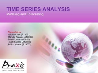

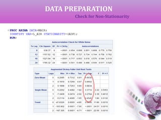
![DATA PREPARATION
Check for Non-Stationarity
If the data is completely random with no fixed pattern, it is called non-
stationary data and cannot be used for future forecasting. This is checked by
‘Augmented Dickey-Fuller Unit Root Test’ (ADF).Here,
H0 : Data is non-stationary
If p < alpha, we reject H0 to claim that the data is stationary and hence
can be used for forecasting.
If p > alpha, we get non-stationary data which can be converted to
stationary by successive differencing.
We can start with first difference (y[t]-y[t-1]) which can obtained using
DIF(L_AIR) or L_AIR(1).Similarly, if we need second difference, it is
DIF2(L_AIR) .](https://image.slidesharecdn.com/timeseriesanalysis-airline-140401030552-phpapp01/85/Time-Series-Analysis-Modeling-and-Forecasting-10-320.jpg)
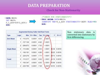
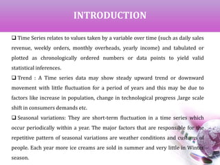
![DATA PREPARATION
Check for Seasonality
The Auto Correlation function (ACF) gives the correlation between y[t]-y[t-s]
where ‘s’ is the period of lag.
If the ACF gives high values at fixed interval, that interval can be considered as the
period of seasonality. A differencing of same order will deseasonalize the data.
In the previous output of ACF as shown below, we can see that 12 years is period of
seasonality.](https://image.slidesharecdn.com/timeseriesanalysis-airline-140401030552-phpapp01/85/Time-Series-Analysis-Modeling-and-Forecasting-13-320.jpg)
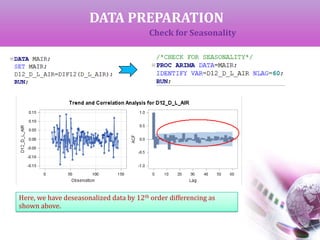
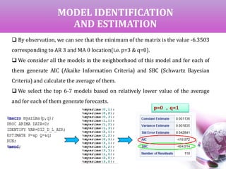
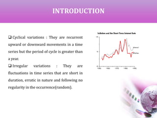
![MODEL IDENTIFICATION
AND ESTIMATION
AIC & SBC for all the neighborhood
models [ (0,1) to (3,3)]
Top 7 models based on lower
average value](https://image.slidesharecdn.com/timeseriesanalysis-airline-140401030552-phpapp01/85/Time-Series-Analysis-Modeling-and-Forecasting-17-320.jpg)
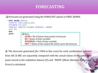
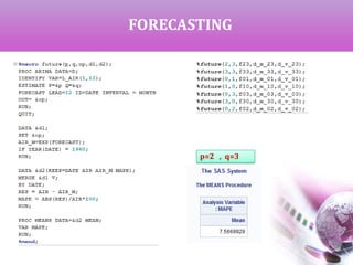
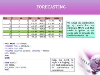
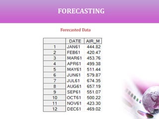
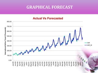


The document presents a time series analysis and forecasting approach by analyzing airline travel data from 1949 to 1960. It covers key concepts such as trends, seasonal variations, and the importance of ensuring data stationarity for effective forecasting. The study utilizes various statistical methods, including transformations and model selection criteria, to generate and compare forecasts against actual values.


![[DSC Europe 25] Raul Cruz Bonilla - Harnessing GEN AI in Fashion, Luxury and ...](https://cdn.slidesharecdn.com/ss_thumbnails/me7nvup5thwqzwzblbvw-raul-cruz-harnessing-ai-en-luxury-260123083019-32ac5a43-thumbnail.jpg?width=640&height=640&fit=bounds)
![[DSC Europe 25] Predrag Maletic - Scaling AI in Banking – Our Strategic Journ...](https://cdn.slidesharecdn.com/ss_thumbnails/qu2onv0aruwlvqtygmxx-predrag-maletic-scaling-ai-in-banking-260123083019-6cf1da1d-thumbnail.jpg?width=640&height=640&fit=bounds)


