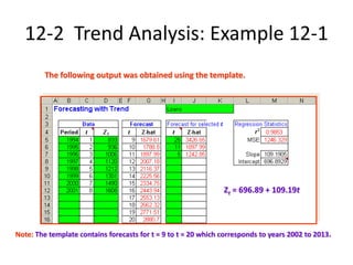
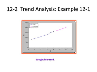
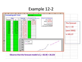
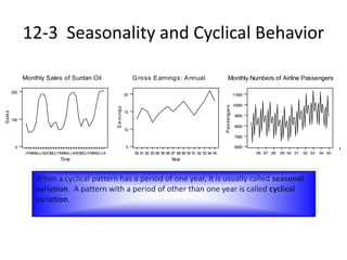
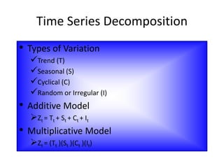
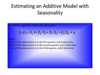
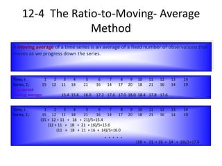
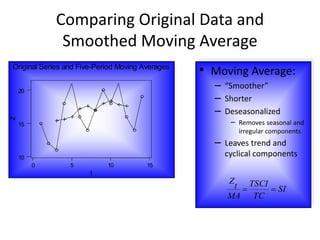
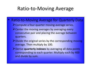
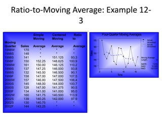
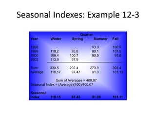
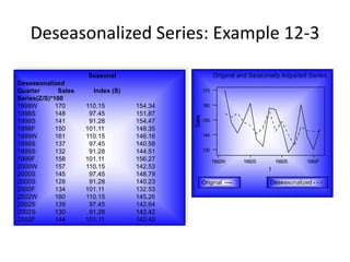
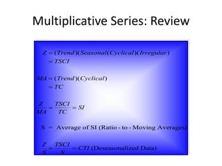
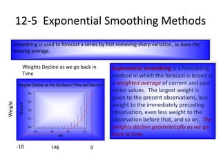
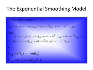
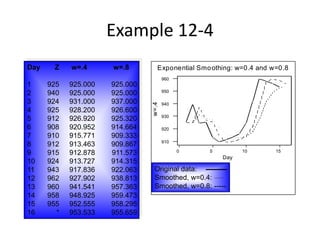
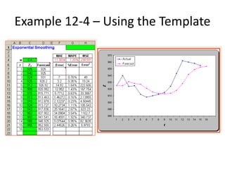
The document provides an overview of time-series forecasting methods, including: 1) It discusses trend analysis, seasonality, cyclical behavior, and various forecasting techniques such as the ratio-to-moving average method and exponential smoothing. 2) Exponential smoothing is described as a forecasting method that gives the largest weight to present observations and smaller, geometrically declining weights to past observations. 3) An example demonstrates exponential smoothing on a time series using weighting factors of 0.4 and 0.8, showing the smoothed series for each weight.

1. TIME-SERIES FORECASTING
Edited By: Dr. Pragati Priyadarshinee, Mumbai,
Mail: pragati.priyadarshinee@welingkar.org

2. • Using Statistics
• Trend Analysis
• Seasonality and Cyclical Behavior
• The Ratio-to-Moving-Average Method
• Exponential Smoothing Methods
• Summary and Review of Terms
Time Series Analysis and Forecasting12

3. A time series is a set of measurements of a variable that are
ordered through time. Time series analysis attempts to detect and
understand regularity in the fluctuation of data over time.
Regular movement of time series data may result from a tendency
to increase or decrease through time - trend- or from a tendency
to follow some cyclical pattern through time - seasonality or
cyclical variation.
Forecasting is the extrapolation of series values beyond the region
of the estimation data. Regular variation of a time series can be
forecast, while random variation cannot.
12-1 Using Statistics

4. A random walk:
Zt- Zt-1=at
or equivalently:
Zt= Zt-1+at
The difference between Z in time t and time t-1 is a random error.
50403020100
15
10
5
0
t
Z
Random Walk
a
There is no evident regularity in a
random walk, since the difference in
the series from period to period is a
random error. A random walk is not
forecastable.
The Random Walk

5. A Time Series as a Superposition of Two Wave
Functions and a Random Error (not shown)
50403020100
4
3
2
1
0
-1
t
z
In contrast with a random walk, this series exhibits obvious cyclical fluctuation. The
underlying cyclical series - the regular elements of the overall fluctuation - may be
analyzable and forecastable.
A Time Series as a Superposition of
Cyclical Functions

6. 12-2 Trend Analysis: Example 12-1
The following output was obtained using the template.
Zt = 696.89 + 109.19t
Note: The template contains forecasts for t = 9 to t = 20 which corresponds to years 2002 to 2013.

7. 12-2 Trend Analysis: Example 12-1
Straight line trend.

8. Example 12-2
Observe that the forecast model is Zt = 82.96 + 26.23t
The forecast
for t = 10
(year 2002)
is 345.27

9. 888786
11000
10000
9000
8000
7000
6000 t
Passengers
Monthly Numbers of Airline Passengers
89 90 91 92 93 94 9595949392919089888786858483828180
20
15
10
5
Year
Earnings
Gross Earnings: Annual
AJJMAMFJDNOSAJJMAMFJDNOSAJJMAMFJ
200
100
0
Time
Sales
Monthly Sales of Suntan Oil
When a cyclical pattern has a period of one year, it is usually called seasonal
variation. A pattern with a period of other than one year is called cyclical
variation.
12-3 Seasonality and Cyclical Behavior

10. • Types of Variation
Trend (T)
Seasonal (S)
Cyclical (C)
Random or Irregular (I)
• Additive Model
Zt = Tt + St + Ct + It
• Multiplicative Model
Zt = (Tt )(St )(Ct )(It)
Time Series Decomposition

11. An additive regression model with seasonality:
Zt=0+ 1 t+ 2 Q1+ 3 Q2 + 4 Q3 + at
where
Q1=1 if the observation is in the first quarter, and 0 otherwise
Q2=1 if the observation is in the second quarter, and 0 otherwise
Q3=1 if the observation is in the third quarter, and 0 otherwise
Estimating an Additive Model with
Seasonality

12. A moving average of a time series is an average of a fixed number of observations that
moves as we progress down the series.
Time, t: 1 2 3 4 5 6 7 8 9 10 11 12 13 14
Series, Zt: 15 12 11 18 21 16 14 17 20 18 21 16 14 19
Five-period
moving average: 15.4 15.6 16.0 17.2 17.6 17.0 18.0 18.4 17.8 17.6
Time, t: 1 2 3 4 5 6 7 8 9 10 11 12 13 14
Series, Zt: 15 12 11 18 21 16 14 17 20 18 21 16 14 19
(15 + 12 + 11 + 18 + 21)/5=15.4
(12 + 11 + 18 + 21 + 16)/5=15.6
(11 + 18 + 21 + 16 + 14)/5=16.0
. . . . .
(18 + 21 + 16 + 14 + 19)/5=17.6
12-4 The Ratio-to-Moving- Average
Method

13. 151050
20
15
10
t
Z
Original Series and Five-Period Moving Averages
• Moving Average:
– “Smoother”
– Shorter
– Deseasonalized
– Removes seasonal and
irregular components
– Leaves trend and
cyclical components
SI
TC
TSCI
MA
t
Z

Comparing Original Data and
Smoothed Moving Average

14. • Ratio-to-Moving Average for Quarterly Data
Compute a four-quarter moving-average series.
Center the moving averages by averaging every
consecutive pair and placing the average between
quarters.
Divide the original series by the corresponding moving
average. Then multiply by 100.
Derive quarterly indexes by averaging all data points
corresponding to each quarter. Multiply each by 400
and divide by sum.
Ratio-to-Moving Average

15. 151050
170
160
150
140
130
Sales
Time
Actual
Smoothed
Actual
Smoothed
MSD:
MAD:
MAPE:
Length:
Moving Average
152.574
10.955
7.816
4
Four-Quarter Moving AveragesSimple Centered Ratio
Moving Moving to
Moving
Quarter Sales Average Average Average
1998W 170 * * *
1998S 148 * * *
1998S 141 * 151.125 93.3
1998F 150 152.25 148.625 100.9
1999W 161 150.00 146.125 110.2
1999S 137 147.25 146.000 93.8
1999S 132 145.00 146.500 90.1
1999F 158 147.00 147.000 107.5
2000W 157 146.00 147.500 106.4
2000S 145 148.00 144.000 100.7
2000S 128 147.00 141.375 90.5
2000F 134 141.00 141.000 95.0
2002W 160 141.75 140.500 113.9
2002S 139 140.25 142.000 97.9
2002S 130 140.75 * *
2002F 144 143.25 * *
Ratio-to-Moving Average: Example 12-
3

16. Quarter
Year Winter Spring Summer Fall
1998 93.3 100.9
1999 110.2 93.8 90.1 107.5
2000 106.4 100.7 90.5 95.0
2002 113.9 97.9
Sum 330.5 292.4 273.9 303.4
Average 110.17 97.47 91.3 101.13
Sum of Averages = 400.07
Seasonal Index = (Average)(400)/400.07
Seasonal
Index 110.15 97.45 91.28 101.11
Seasonal Indexes: Example 12-3

17. Seasonal
Deseasonalized
Quarter Sales Index (S)
Series(Z/S)*100
1998W 170 110.15 154.34
1998S 148 97.45 151.87
1998S 141 91.28 154.47
1998F 150 101.11 148.35
1999W 161 110.15 146.16
1999S 137 97.45 140.58
1999S 132 91.28 144.51
1999F 158 101.11 156.27
2000W 157 110.15 142.53
2000S 145 97.45 148.79
2000S 128 91.28 140.23
2000F 134 101.11 132.53
2002W 160 110.15 145.26
2002S 139 97.45 142.64
2002S 130 91.28 142.42
2002F 144 101.11 142.42
Original Deseasonalized - - -
1992F1992S1992S1992W
170
160
150
140
130
t
Sales
Original and Seasonally Adjusted Series
Deseasonalized Series: Example 12-3

18. 180
170
160
150
140
130
120
1992F1992S1992S1992W
t
Sales
Trend Line and Moving Averages The cyclical component is the
remainder after the moving averages
have been detrended. In this
example, a comparison of the moving
averages and the estimated
regression line:
illustrates that the cyclical
component in this series is negligible.
 . .Z t 155275 11059
The Cyclical Component: Example 12-3

19. The centered moving average, ratio to moving average, seasonal index, and
deseasonalized values were determined using the Ratio-to-Moving-Average method.
Example 12-3 using the Template
This displays just a
partial output for the
quarterly forecasts.

20. Example 12-3 using the Template
Graph of the quarterly Seasonal Index

21. Example 12-3 using the Template
Graph of the Data and the quarterly Forecasted values

22. The centered moving average, ratio to moving average, seasonal index, and
deseasonalized values were determined using the Ratio-to-Moving-Average method.
Example 12-3 using the Template
This displays just a
partial output for the
monthly forecasts.

23. Example 12-3 using the Template
Graph of the monthly Seasonal Index

24. Example 12-3 using the Template
Graph of the Data and the monthly Forecasted values

25. 152.02=)(1.1015)(1)(138.03=
=ˆ
e)(negligibl1C
1.1015=S
138.03=)(0.837)(17-152.26=zˆ:Trend
:17)=(t2002for WinterForecast
=ˆ
:seriestivemultiplicaaofforecastThe
TSCZ
TSCZ

Forecasting a Multiplicative Series:
Example 12-3

26. Z Trend Seasonal Cyclical Irregular
TSCI
MA Trend Cyclical
TC
Z
MA
TSCI
TC
SI
Z
S
TSCI
S
CTI




 
 
( )( ( )( )
( )( )
S = Average of SI (Ratio - to - Moving Averages)
(Deseasonalized Data)
Multiplicative Series: Review

27. Smoothing is used to forecast a series by first removing sharp variation, as does the
moving average.
Exponential smoothing is a forecasting
method in which the forecast is based in
a weighted average of current and past
series values. The largest weight is
given to the present observations, less
weight to the immediately preceding
observation, even less weight to the
observation before that, and so on. The
weights decline geometrically as we go
back in time.
0-5-10-15
0.4
0.3
0.2
0.1
0.0
Lag
Weight
Weights Decline as We Go BackinTime and Sumto 1
Weights Decline as we go back in
Time
-10 0
Weight
Lag
12-5 Exponential Smoothing Methods

28. Given a weighting factor: < < :
Since
So
0 1
1 1 1 1
2
2 1
3
3
1 1 2 1
2
3 1
3
4
1 1 1 1
2
2 1
3
3
w
Zt w Zt w w Zt w w Zt w w Zt
Zt w Zt w w Zt w w Zt w w Zt
w Zt w w Zt w w Zt w w Zt
 ( ) ( )( ) ( ) ( ) ( ) ( )
 ( ) ( )( ) ( ) ( ) ( ) ( )
( )  ( )( ) ( ) ( ) ( ) ( )

           
           
          
 



Zt 1 w(Zt ) (1 w)(Zt )
Zt 1 Zt (1 w)(Zt - Zt )
 
   

 
The Exponential Smoothing Model

29. Day Z w=.4 w=.8
1 925 925.000 925.000
2 940 925.000 925.000
3 924 931.000 937.000
4 925 928.200 926.600
5 912 926.920 925.320
6 908 920.952 914.664
7 910 915.771 909.333
8 912 913.463 909.867
9 915 912.878 911.573
10 924 913.727 914.315
11 943 917.836 922.063
12 962 927.902 938.813
13 960 941.541 957.363
14 958 948.925 959.473
15 955 952.555 958.295
16 * 953.533 955.659
Original data:
Smoothed, w=0.4: ......
Smoothed, w=0.8: -----
Day
151050
960
950
940
930
920
910
w=.4
Exponential Smoothing: w=0.4 and w=0.8
Example 12-4

30. Example 12-4 – Using the Template