The normal distribution

The Normal Distribution

Slide 1

Shakeel Nouman
M.Phil Statistics

The Normal Distribution By Shakeel Nouman M.Phil Statistics Govt. College University Lahore, Statistical Officer

4











Slide 2

The Normal Distribution

Using Statistics
The Normal Probability Distribution
The Standard Normal Distribution
The Transformation of Normal Random
Variables
The Inverse Transformation
The Normal Distribution as an
Approximation to Other Probability
Distributions
Summary and Review of Terms


4-1 Introduction

Slide 3

As n increases, the binomial distribution approaches a ...
n=6

n = 10

Bino mial Dis trib utio n: n=6, p =.5

n = 14

Bino mial Distrib utio n: n=1 0 , p =.5

Bino mial Dis trib utio n: n=1 4 , p =.5
0.3

0.2

0.2

0.2

0.1

P(x)

0.3

P(x)

P(x)

0.3

0.1

0.0

0.1

0.0
0

1

2

3

4

5

6

0.0
0

1

x

2

3

4

5

6

7

8

9

10

0 1 2 3 4 5 6 7 8 9 10 11 12 13 14

x

x

Normal Probability Density Function:
f ( x) 

1






 x
2
2p
where e  2.7182818... and p  314159265...
.

0.4
0.3

f(x)

x  2

e 2 2 for






Normal Distribution:  = 0,= 1

0.2
0.1
0.0
-5

0

x


5

The Normal Probability
Distribution

Slide 4

The normal probability density function:
1

e

0.4

x  2





2 2

0.3

for

 x

2p 2
where e  2.7182818... and p  314159265...
.

f(x)

f ( x) 









Normal Dis tribution:  = 0,= 1

0.2
0.1
0.0
-5

0

x


5

Properties of the Normal
Probability Distribution
•

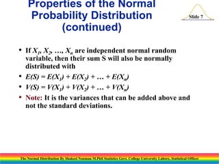
Slide 5

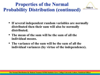
The normal is a family of
Bell-shaped and symmetric distributions. because the
distribution is symmetric, one-half (.50 or 50%) lies
on either side of the mean.
Each is characterized by a different pair of mean, ,


and variance,  . That is: [X~N( )].
Each is asymptotic to the horizontal axis.
The area under any normal probability density
function within kof is the same for any normal
distribution, regardless of the mean and variance.


Probability Distribution (continued)
•
•
•

Slide 6

If several independent random variables are normally
distributed then their sum will also be normally
distributed.
The mean of the sum will be the sum of all the
individual means.
The variance of the sum will be the sum of all the
individual variances (by virtue of the independence).


Probability Distribution
(continued)
•
•
•
•

Slide 7

If X1, X2, …, Xn are independent normal random
variable, then their sum S will also be normally
distributed with
E(S) = E(X1) + E(X2) + … + E(Xn)
V(S) = V(X1) + V(X2) + … + V(Xn)
Note: It is the variances that can be added above and
not the standard deviations.


Probability Distribution – Example
4-1

Slide 8

Example 4.1: Let X1, X2, and X3 be independent random
variables that are normally distributed with means and
variances as shown.
Mean

Variance

X1

10

1

X2

20

2

X3

30

3

Let S = X1 + X2 + X3. Then E(S) = 10 + 20 + 30 = 60 and
V(S) = 1 + 2 + 3 = 6. The standard deviation of S 6
is
= 2.45.

Properties
of
the
Normal
Probability Distribution (continued)
•

•
•
•

Slide 9

If X1, X2, …, Xn are independent normal random
variable, then the random variable Q defined as Q =
a1X1 + a2X2 + … + anXn + b will also be normally
distributed with
E(Q) = a1E(X1) + a2E(X2) + … + anE(Xn) + b
V(Q) = a12 V(X1) + a22 V(X2) + … + an2 V(Xn)
Note: It is the variances that can be added above and
not the standard deviations.


Probability Distribution – Example
4-3

Slide 10

Example 4.3: Let X1 , X2 , X3 and X4 be independent random variables
that are normally distributed with means and variances as shown.
Find the mean and variance of Q = X1 - 2X2 + 3X2 - 4X4 + 5
Mean

Variance

X1

12

4

X2

-5

2

X3

8

5

X4

10

1

E(Q) = 12 – 2(-5) + 3(8) – 4(10) + 5 = 11

V(Q) = 4 + (-2)2(2) + 32(5) + (-4)2(1) = 73
SD(Q) =

73  8.544


Computing the Mean, VarianceSlide 11
and Standard Deviation for the
Sum of Independent Random
Variables Using the Template


Normal Probability Distributions

Slide 12

All of these are normal probability density functions, though each has a different mean and variance.
Normal Distribution: =40, 
=1

=5

0.4

=3

0.2

0.2

0.2

f(y)

f(x)

f(w)

0.3
0.1

0.1

0.1
0.0

0.0
35

40

45

0.0
0

w

10

20

30

40

50

x

W~N(40,1)

X~N(30,25)

60

35

45

50

55

y

Y~N(50,9)

Normal Distribution:  
=0, =1

Consider:

0.4

f(z)

0.3
0.2
0.1
0.0
-5

0

5

P(39 W 41)
P(25 X 35)
P(47 Y 53)
P(-1 Z 1)

The probability in each
case is an area under a
normal probability density
function.

z

Z~N(0,1)

65

Computing Normal Probabilities
Using the Template

Slide 13


4-3 The Standard Normal
Distribution

Slide 14

The standard normal random variable, Z, is the normal random
variable with mean = 0 and standard deviation = 1:
Z~N(0,12).
Standard Normal Distribution
0 .4


=1

{

f( z)

0 .3

0 .2

0 .1

0 .0
-5

-4

-3

-2

-1

0

1

2

3

4

5


=0
Z


Finding Probabilities of the
Standard Normal Distribution: P(0
< Z < 1.56)

Slide 15

Standard Normal Probabilities
0.4

f(z)

0.3
0.2
0.1

{

1.56

0.0
-5

-4

-3

-2

-1

0

1

2

3

4

5

Z

Look in row labeled 1.5
and column labeled .06 to
find P(0 z 1.56) =
.4406

z
0.0
0.1
0.2
0.3
0.4
0.5
0.6
0.7
0.8
0.9
1.0
1.1
1.2
1.3
1.4
1.5
1.6
1.7
1.8
1.9
2.0
2.1
2.2
2.3
2.4
2.5
2.6
2.7
2.8
2.9
3.0

.00
0.0000
0.0398
0.0793
0.1179
0.1554
0.1915
0.2257
0.2580
0.2881
0.3159
0.3413
0.3643
0.3849
0.4032
0.4192
0.4332
0.4452
0.4554
0.4641
0.4713
0.4772
0.4821
0.4861
0.4893
0.4918
0.4938
0.4953
0.4965
0.4974
0.4981
0.4987

.01
0.0040
0.0438
0.0832
0.1217
0.1591
0.1950
0.2291
0.2611
0.2910
0.3186
0.3438
0.3665
0.3869
0.4049
0.4207
0.4345
0.4463
0.4564
0.4649
0.4719
0.4778
0.4826
0.4864
0.4896
0.4920
0.4940
0.4955
0.4966
0.4975
0.4982
0.4987

.02
0.0080
0.0478
0.0871
0.1255
0.1628
0.1985
0.2324
0.2642
0.2939
0.3212
0.3461
0.3686
0.3888
0.4066
0.4222
0.4357
0.4474
0.4573
0.4656
0.4726
0.4783
0.4830
0.4868
0.4898
0.4922
0.4941
0.4956
0.4967
0.4976
0.4982
0.4987

.03
0.0120
0.0517
0.0910
0.1293
0.1664
0.2019
0.2357
0.2673
0.2967
0.3238
0.3485
0.3708
0.3907
0.4082
0.4236
0.4370
0.4484
0.4582
0.4664
0.4732
0.4788
0.4834
0.4871
0.4901
0.4925
0.4943
0.4957
0.4968
0.4977
0.4983
0.4988

.04
0.0160
0.0557
0.0948
0.1331
0.1700
0.2054
0.2389
0.2704
0.2995
0.3264
0.3508
0.3729
0.3925
0.4099
0.4251
0.4382
0.4495
0.4591
0.4671
0.4738
0.4793
0.4838
0.4875
0.4904
0.4927
0.4945
0.4959
0.4969
0.4977
0.4984
0.4988

.05
0.0199
0.0596
0.0987
0.1368
0.1736
0.2088
0.2422
0.2734
0.3023
0.3289
0.3531
0.3749
0.3944
0.4115
0.4265
0.4394
0.4505
0.4599
0.4678
0.4744
0.4798
0.4842
0.4878
0.4906
0.4929
0.4946
0.4960
0.4970
0.4978
0.4984
0.4989

.06
0.0239
0.0636
0.1026
0.1406
0.1772
0.2123
0.2454
0.2764
0.3051
0.3315
0.3554
0.3770
0.3962
0.4131
0.4279
0.4406
0.4515
0.4608
0.4686
0.4750
0.4803
0.4846
0.4881
0.4909
0.4931
0.4948
0.4961
0.4971
0.4979
0.4985
0.4989

.07
0.0279
0.0675
0.1064
0.1443
0.1808
0.2157
0.2486
0.2794
0.3078
0.3340
0.3577
0.3790
0.3980
0.4147
0.4292
0.4418
0.4525
0.4616
0.4693
0.4756
0.4808
0.4850
0.4884
0.4911
0.4932
0.4949
0.4962
0.4972
0.4979
0.4985
0.4989

.08
0.0319
0.0714
0.1103
0.1480
0.1844
0.2190
0.2517
0.2823
0.3106
0.3365
0.3599
0.3810
0.3997
0.4162
0.4306
0.4429
0.4535
0.4625
0.4699
0.4761
0.4812
0.4854
0.4887
0.4913
0.4934
0.4951
0.4963
0.4973
0.4980
0.4986
0.4990


.09
0.0359
0.0753
0.1141
0.1517
0.1879
0.2224
0.2549
0.2852
0.3133
0.3389
0.3621
0.3830
0.4015
0.4177
0.4319
0.4441
0.4545
0.4633
0.4706
0.4767
0.4817
0.4857
0.4890
0.4916
0.4936
0.4952
0.4964
0.4974
0.4981
0.4986
0.4990

Standard Normal Distribution: P(Z
< -2.47)
To find P(Z<-2.47):
Find table area for 2.47
P(0 < Z < 2.47) = .4932

P(Z < -2.47) = .5 - P(0 < Z < 2.47)

z ...
.
.
.
2.3 ...
2.4 ...
2.5 ...

Slide 16

.06
.07
.08
.
.
.
.
.
.
.
.
.
0.4909 0.4911 0.4913
0.4931 0.4932 0.4934
0.4948 0.4949 0.4951
.
.
.

= .5 - .4932 = 0.0068


Area to the left of -2.47
P(Z < -2.47) = .5 - 0.4932
= 0.0068

0.4

Table area for 2.47
P(0 < Z < 2.47) = 0.4932

f(z)

0.3

0.2

0.1

0.0
-5

-4

-3

-2

-1

0

1

2

3

4

5

Z


Standard Normal Distribution:
P(1< Z < 2)
To find P(1  Z  2):
1. Find table area for 2.00
F(2)  P(Z  2.00)  .5 + .4772 .9772
2. Find table area for 1.00
F(1)  P(Z  1.00)  .5 + .3413  .8413
3. P(1  Z  2.00)  P(Z  2.00)  P(Z  1.00)

z

.00
.
.
.

0.9
1.0
1.1
.
.
.
1.9
2.0
2.1

 .9772  .8413  .1359

.
.
.

.
.
.
0.3159
0.3413
0.3643
.
.
.
0.4713
0.4772
0.4821
.
.
.

Slide 17

...

...
...
...

...
...
...

0.4

Area between 1 and 2
P(1  Z  2)  .9772  .8413  0.1359

f(z)

0.3

0.2

0.1

0.0
-5

-4

-3

-2

-1

0

1

2

3

4

5

Z


Finding Values of the Standard
Normal Random Variable: P(0 < Z
< z) = 0.40
To find z such that
P(0 Z z) = .40:
1. Find a probability as close as
possible to .40 in the table of
standard normal probabilities.

z
0.0
0.1
0.2
0.3
0.4
0.5
0.6
0.7
0.8
0.9
1.0
1.1
1.2
1.3
.
.
.

.00
0.0000
0.0398
0.0793
0.1179
0.1554
0.1915
0.2257
0.2580
0.2881
0.3159
0.3413
0.3643
0.3849
0.4032
.
.
.

.01
0.0040
0.0438
0.0832
0.1217
0.1591
0.1950
0.2291
0.2611
0.2910
0.3186
0.3438
0.3665
0.3869
0.4049
.
.
.

.02
0.0080
0.0478
0.0871
0.1255
0.1628
0.1985
0.2324
0.2642
0.2939
0.3212
0.3461
0.3686
0.3888
0.4066
.
.
.

2. Then determine the value of z
from the corresponding row
and column.

.03
0.0120
0.0517
0.0910
0.1293
0.1664
0.2019
0.2357
0.2673
0.2967
0.3238
0.3485
0.3708
0.3907
0.4082
.
.
.

.04
0.0160
0.0557
0.0948
0.1331
0.1700
0.2054
0.2389
0.2704
0.2995
0.3264
0.3508
0.3729
0.3925
0.4099
.
.
.

.05
0.0199
0.0596
0.0987
0.1368
0.1736
0.2088
0.2422
0.2734
0.3023
0.3289
0.3531
0.3749
0.3944
0.4115
.
.
.

.06
0.0239
0.0636
0.1026
0.1406
0.1772
0.2123
0.2454
0.2764
0.3051
0.3315
0.3554
0.3770
0.3962
0.4131
.
.
.

Slide 18

.07
0.0279
0.0675
0.1064
0.1443
0.1808
0.2157
0.2486
0.2794
0.3078
0.3340
0.3577
0.3790
0.3980
0.4147
.
.
.

.08
0.0319
0.0714
0.1103
0.1480
0.1844
0.2190
0.2517
0.2823
0.3106
0.3365
0.3599
0.3810
0.3997
0.4162
.
.
.

0.4

Area to the left of 0 = .50

P(0 Z 1.28)  .40P(z 0) = .50

f(z)

Also, since P(Z 0) = .50

Area = .40 (.3997)

0.3

0.2

0.1

P(Z 1.28)  .90
0.0

-5

-4

-3

-2

-1

0

Z

1

2

3

4

5

Z = 1.28


.09
0.0359
0.0753
0.1141
0.1517
0.1879
0.2224
0.2549
0.2852
0.3133
0.3389
0.3621
0.3830
0.4015
0.4177
.
.
.

99% Interval around the Mean
To have .99 in the center of the distribution, there
should be (1/2)(1-.99) = (1/2)(.01) = .005 in each
tail of the distribution, and (1/2)(.99) = .495 in
each half of the .99 interval. That is:

P(0 Z z.005) = .495

z

.04

.

.
.
.
2.4 ...
2.5 ...
2.6 ...
.
.
.

.05

.08

.
.
.
0.4931
0.4948
0.4961
.
.
.

.09

.
.
.
0.4932
0.4949
0.4962
.
.
.

.
.
.
0.4934
0.4951
0.4963
.
.
.

.
.
0.4936
0.4952
0.4964
.
.
.

Total area in center = .99

Area in center left = .495
0.4

Area in center right = .495
0.3

f(z)

P(-.2575   .99
Z
)=

.07

.
.
.
0.4929
0.4946
0.4960
.
.
.

Look to the table of standard normal probabilities
to find that:

  
z.005
z.005 

.06

.
.
.
0.4927
0.4945
0.4959
.
.
.

Slide 19

0.2

Area in right tail = .005
Area in left tail = .005

0.1

0.0
-5

-4

-3

-2

-z.005
-2.575

-1

0

Z

1

2

3

4

5

z.005
2.575


4-4 The Transformation of
Normal Random Variables

Slide 20

The area within k of the mean is the same for all normal random variables. So an area
under any normal distribution is equivalent to an area under the standard normal. In this
example: P(40 X 
P(-1 Z  
since m = 50 and s = 10.
The transformation of X to Z:
X x
Z
x

Normal Distribution:=50,
=10
0.07
0.06

Transformation
f(x)

(1) Subtraction: (X -  )
x

0.05
0.04
0.03
 10
=

{

0.02


0.01
0.00

0.4

0

20

30

40

50

60

70

80

90 100

X

0.3

0.2

(2) Division by  )
x

{

f(z)

10

1.0

0.1

0.0
-5

-4

-3

-2

-1

0

Z

1

2

3

4

5

The inverse transformation of Z to X:

X  x + Z x


Using the Normal
Transformation

Example 4-9
X~N(160,302)

Slide 21

Example 4-10
X~N(127,222)

P (100  X  180)
 100    X    180   
 P


P ( X  150)
 X    150   
 P






 

 
 100  160  Z  180  160
P

 30
30 

(

)

 P 2  Z  .6667
 0.4772 + 0.2475  0.7247

 
 
 150  127 
P Z 


22 

(

)

 P Z  1.045
 0.5 + 0.3520  0.8520


Using the Normal
Transformation - Example 4-11

Normal Dis tribution:  = 383, = 12

Example 4-11
X~N(383,122)

0.05
0.04

(

 
399  383

)

12

 P 0.9166  Z  1.333
 0.4088  0.3203  0.0885




0.03
0.02
0.01

0.00
340

0.4

390

X
0.3

f(z)



f( )
X

P ( 394  X  399)
 394   X   399   
 P




 

 394  383
P
Z 
 12

Slide 22

0.2

0.1

0.0
-5

-4

-3

-2

-1

0

1

2

3

4

5

Z

Template solution


440

The Transformation of Normal
Random Variables
The transformation of X to Z:
Z 

X  x

x

Slide 23

The inverse transformation of Z to X:
X  

+ Z
x

x

The transformation of X to Z, where a and b are numbers::

a  

P( X  a)  P Z 


 
b  

P( X  b)  P Z 


 
b  
a 
P(a  X  b)  P
Z

 
 


Normal
Rule)

Probabilities

(Empirical

S t a n d a rd N o rm a l D is trib u tio n

• The probability that a normal

•

•

0 .4

0 .3

f(z)

random variable will be within 1
standard deviation from its mean
(on either side) is 0.6826, or
approximately 0.68.
The probability that a normal
standard deviations from its mean
is 0.9544, or approximately 0.95.
The probability that a normal
standard deviation from its mean is
0.9974.

Slide 24

0 .2

0 .1

0 .0
-5

-4

-3

-2

-1

0

1

2

3

Z


4

5

4-5 The Inverse Transformation

Slide 25

The area within k of the mean is the same for all normal random variables. To find a
probability associated with any interval of values for any normal random variable, all that
is needed is to express the interval in terms of numbers of standard deviations from the
mean. That is the purpose of the standard normal transformation. If X~N(50,102),
70  50 
 x   70   

P( X  70)  P

  P Z 
  P( Z  2)
 

 
10 

That is, P(X >70) can be found easily because 70 is 2 standard deviations above the mean
of X: 70 = + 2 P(X > 70) is equivalent to P(Z > 2), an area under the standard normal
.
distribution.
Normal Distribution:  = 124, = 12

Example 4-12
X~N(124,122)
P(X > x) = 0.10 and P(Z > 1.28) 
0.10
x = + z= 124 + (1.28)(12) =
139.36
.
.
.
1.1
1.2
1.3

.
.
.

.07
.
.
.
0.3790
0.3980
0.4147

.
.
.
...
...
...

.
.
.

.
.
.

.08
.
.
.
0.3810
0.3997
0.4162

.
.
.

.09
.
.
.
0.3830
0.4015
0.4177

.
.
.

0.03

f(x)

z

0.04

0.02

0.01

0.01

0.00
80

130

X

139.36


180

Template Solution for Example
4-12

Slide 26

Example 4-12
X~N(124,122)
P(X > x) = 0.10 and P(Z > 1.28) 
0.10
x = + z= 124 + (1.28)(12) =
139.36


The Inverse Transformation
(Continued)
Example 4-13
X~N(5.7,0.52)
P(X > x)=0.01 and P(Z > 2.33) 
0.01
x = + z= 5.7 + (2.33)(0.5) = 6.865
z
.
.
.
2.2
2.3
2.4
.
.
.

.02
.
.
.
0.4868
0.4898
0.4922

.
.
.
...
...
...
.
.
.

.03
.
.
.
0.4871
0.4901
0.4925

.
.
.

.
.
.

Example 4-14
X~N(2450,4002)
P(a<X<b)=0.95 and P(-1.96<Z<1.96)
0.95
x = z= 2450 (1.96)(400) = 2450
784=(1666,3234)
P(1666 < X < 3234) = 0.95

.04
.
.
.
0.4875
0.4904
0.4927

z
.
.
.
1.8
1.9
2.0
.

.
.
.

Normal Distribution: = 5.7  0.5
=

...
...
...
.
.

.06
.
.
.
0.4686
0.4750
0.4803
.

.

.

0.0015

Area = 0.49

.4750

.4750

0.0010

f(x)

0.5
0.4
X.01 = 
+z= 5.7 + (2.33)(0.5) = 6.865

0.3

0.0005

0.2

.0250

.0250

Area = 0.01

0.1
0.0

0.0000
3.2

4.2

5.2

6.2

7.2

8.2

1000

2000

X
-5

-4

-3

-2

-1

0

z

3000

4000

X
1

2

3

4

5

Z.01 = 2.33

-5

-4

-3

-2

-1.96

-1

0

Z

1

2

3

.07
.
.
.
0.4693
0.4756
0.4808
.
.

Normal Distribution:  = 2450 = 400

0.6

f(x)

.05
.
.
.
0.4678
0.4744
0.4798
.

.
.
.

.

0.8
0.7

Slide 27

4

5

1.96


Finding Values of a Normal
Random Variable, Given a
Probability
Norm al Distribution:  = 24 50, = 40 0
0.0012
.
0.0010
.
0.0008
.

f(x)

1. Draw pictures of
the normal
distribution in
question and of the
standard normal
distribution.

Slide 28

0.0006
.
0.0004
.
0.0002
.
0.0000
1000

2000

3000

4000

X

S ta nd a rd N o rm al D is trib utio n
0.4

f(z)

0.3
0.2
0.1
0.0
-5

-4

-3

-2

-1

0

1

2

3

4

5

Z


Probability
Norm al Distribution:  = 24 50, = 400
0.0012
.

.4750

0.0010
.

.4750

0.0008
.

f(x)

1. Draw pictures of
the
normal
distribution
in
question and of the
standard normal
distribution.

Slide 29

0.0006
.
0.0004
.
0.0002
.

.9500

0.0000
1000

2000

3000

4000

X

2. Shade the area
corresponding to
the
desired
probability.

S ta nd a rd No rm al D is trib utio n
0.4

.4750

.4750

f(z)

0.3
0.2
0.1

.9500

0.0
-5

-4

-3

-2

-1

0

1

2

3

4

5

Z


Probability
Norm al Distribution:  = 2450, = 400

3. From the table
of the standard
normal
distribution,
find the z value
or values.

0.0012
.

.4750

0.0010
.

.4750

0.0008
.

f(x)

1. Draw pictures of
the normal
distribution in
question and of the
standard normal
distribution.

Slide 30

0.0006
.
0.0004
.
0.0002
.

.9500

0.0000
1000

2000

3000

4000

X

2. Shade the area
corresponding
to the desired
probability.

0.4

.4750

f(z)
z
.
.
.
1.8
1.9
2.0
.
.

.05
.
.
.
0.4678
0.4744
0.4798
.

.
.
.
...
...
...
.
.

.

.06
.
.
.
0.4686
0.4750
0.4803
.
.

.4750

0.3

.07
.
.
.
0.4693
0.4756
0.4808
.

0.2
0.1

.9500

0.0
-5

-4

-3

-2

-1

0

1

2

3

4

5

Z

.

-1.96

1.96


Probability
Norm al Distribution:  = 24 50, = 400

3. From the table
of the standard
normal
distribution,
find the z value
or values.

0.0012
.

.4750

0.0010
.

.4750

0.0008
.

f(x)

1. Draw pictures of
the normal
distribution in
question and of the
standard normal
distribution.

Slide 31

0.0006
.
0.0004
.
0.0002
.

.9500

0.0000
1000

2000

3000

4000

X

2. Shade the area
corresponding
to the desired
probability.

0.4

.4750

.
.
.
...
...
...
.
.

.05
.
.
.
0.4678
0.4744
0.4798
.
.

.06
.
.
.
0.4686
0.4750
0.4803
.
.

.4750

0.3

f(z)
z
.
.
.
1.8
1.9
2.0
.
.

4. Use the
transformation
from z to x to get
value(s) of the
original random
variable.


.07
.
.
.
0.4693
0.4756
0.4808
.
.

0.2
0.1

.9500

0.0
-5

-4

-3

-2

-1

0

1

2

Z

-1.96

3

4

5

x = z= 2450
(1.96)(400)
= 2450 784=(1666,3234)

1.96


Probability

Slide 32

The normal distribution with = 3.5 and = 1.323 is a close
approximation to the binomial with n = 7 and p = 0.50.
P(x<4.5) = 0.7749

Normal Distribution:  = 3.5, = 1.323

Binomial Distribution: n = 7, p = 0.50

0.3

0.3

P( x  = 0.7734
4)
0.2

f(x)

P(x)

0.2

0.1

0.1

0.0

0.0
0

5

10

X

0

1

2

3

4

5

6

7

X

MTB > cdf 4.5;
SUBC> normal 3.5 1.323.
Cumulative Distribution Function

MTB > cdf 4;
SUBC> binomial 7,.5.

Normal with mean = 3.50000 and standard deviation = 1.32300

Binomial with n = 7 and p = 0.500000

x P( X <= x)
4.5000
0.7751

x P( X <= x)
4.00
0.7734


4-6 The Normal Approximation of
Binomial Distribution

Slide 33

The normal distribution with = 5.5 and = 1.6583 is a closer
approximation to the binomial with n = 11 and p = 0.50.
P(x < 4.5) = 0.2732
Normal Distribution: = 5.5, = 1.6583

Binomial Distribution: n = 11, p = 0.50

P(x 4) = 0.2744

0.3
0.2

f(x)

P(x)

0.2
0.1

0.1

0.0

0.0
0

5

10

X

MTB > cdf 4.5;
SUBC> normal 5.5 1.6583.
Normal with mean = 5.50000 and standard deviation = 1.65830
x P( X <= x)
4.5000
0.2732

0

1

2

3

4

5

6

7

8

9 10 11

X

MTB > cdf 4;
SUBC> binomial 11,.5.
Binomial with n = 11 and p = 0.500000
x P( X <= x)
4.00
0.2744


Approximating a Binomial
Probability Using the Normal
Distribution

Slide 34

b  np 
 a  np
P ( a  X  b)  P 
Z


 np(1  p)
np(1  p) 
for n large (n  50) and p not too close to 0 or 1.00
or:

b + 0.5  np 
 a  0.5  np
P ( a  X  b)  P 
Z


np(1  p) 
 np(1  p)
for n moderately large (20  n < 50).

If p is either small (close to 0) or large (close to 1), use the Poisson
approximation.

Using the Template for Normal
Approximation of the Binomial
Distribution

Slide 35


Name
Religion
Domicile
Contact #
E.Mail
M.Phil (Statistics)

Shakeel Nouman
Christian
Punjab (Lahore)
0332-4462527. 0321-9898767
sn_gcu@yahoo.com
sn_gcu@hotmail.com
GC University, .
(Degree awarded by GC University)

M.Sc (Statistics)
Statitical Officer
(BS-17)
(Economics & Marketing
Division)

GC University, .
(Degree awarded by GC University)

Livestock Production Research Institute
Bahadurnagar (Okara), Livestock & Dairy Development
Department, Govt. of Punjab


The normal distribution

Recommended

Recommended

More Related Content

What's hot

What's hot (20)

Viewers also liked

Viewers also liked (9)

Similar to The normal distribution

Similar to The normal distribution (20)

More from Shakeel Nouman

More from Shakeel Nouman (14)

Recently uploaded

Recently uploaded (20)

The normal distribution