Download to read offline

![Confidence Intervals for Paired
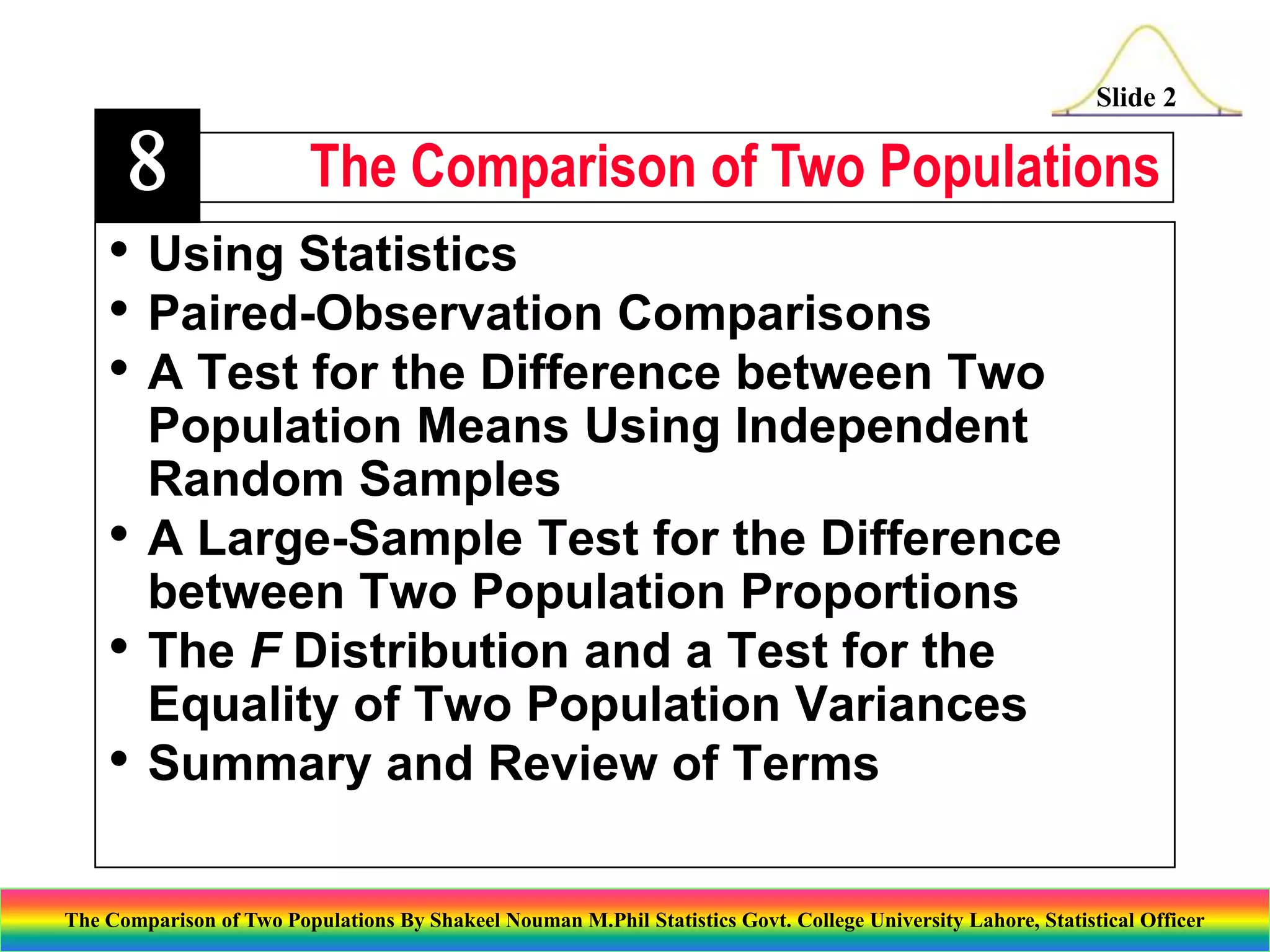
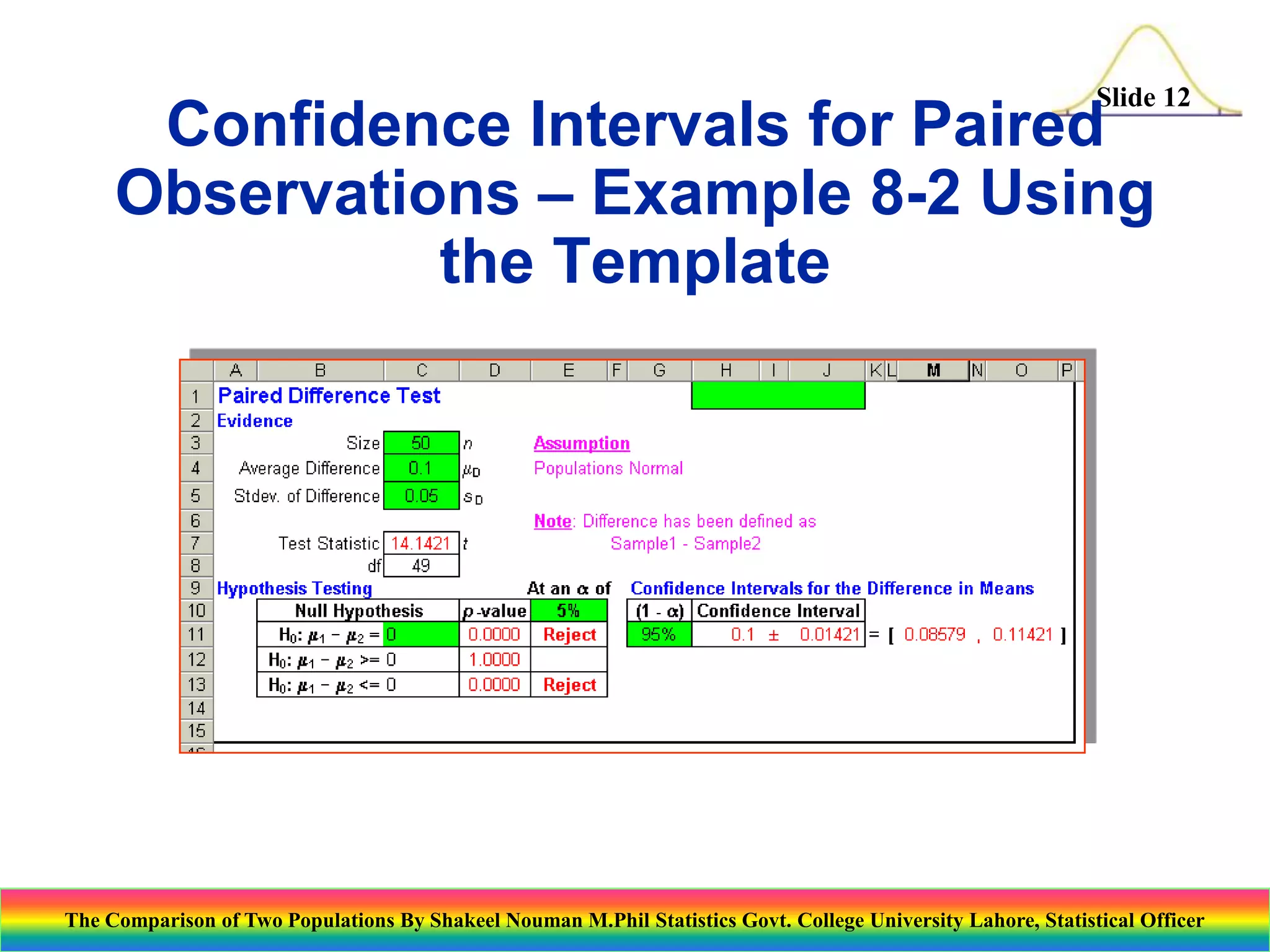
Observations – Example 8-2
Slide 11
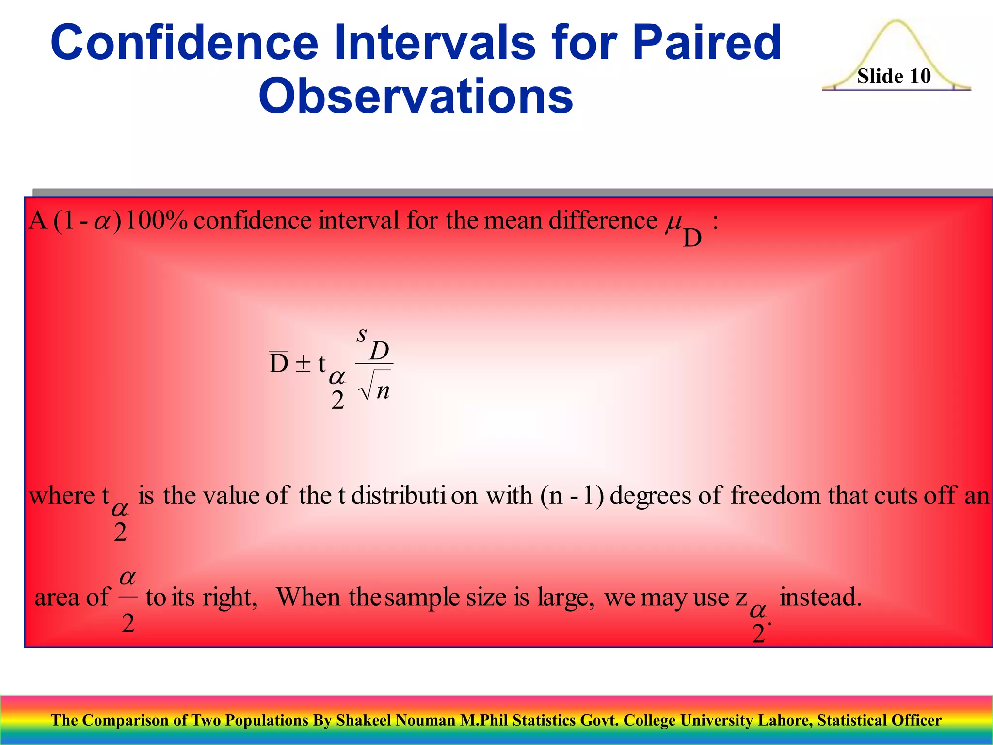
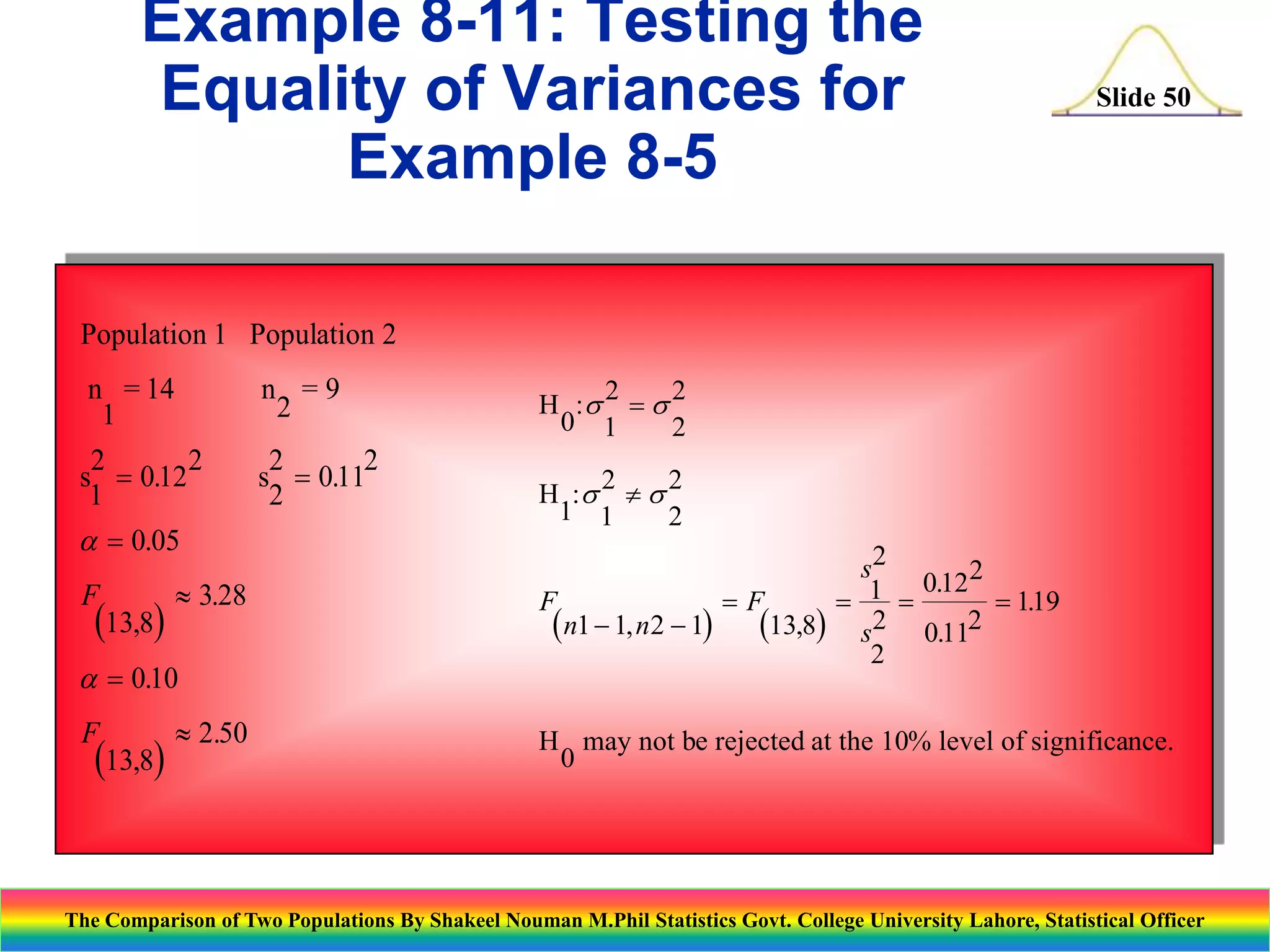
95% confidence interval for the data in Example 8 - 2 :
s
D z D 0.11.96 0.05 0.1 (1.96)(.0071)
n
50
2
0.1 0.014 [0.086,0.114]
Note that this confidence interval does not include the value 0.
The Comparison of Two Populations By Shakeel Nouman M.Phil Statistics Govt. College University Lahore, Statistical Officer](https://image.slidesharecdn.com/thecomparisonoftwopopulations-140129013701-phpapp02/75/The-comparison-of-two-populations-11-2048.jpg)
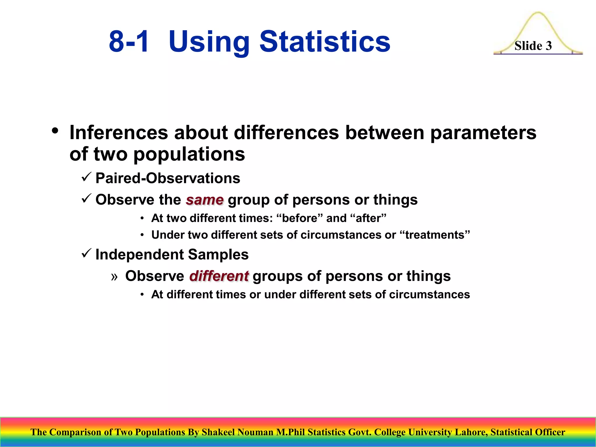
![Confidence Intervals for the
Difference between Two
Population Means
Slide 21
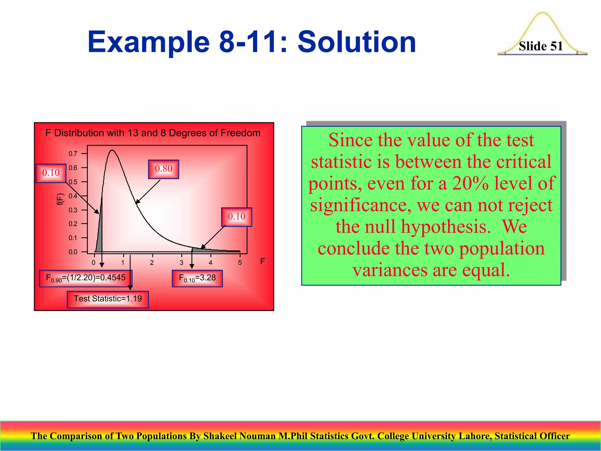
A large-sample (1-)100% confidence interval for the difference
between two population means, 1- 2 , using independent
random samples:
(x - x ) z
1
2
2
2
2
s
1 + 2
n
n
1
2
s
A 95% confidence interval using the data in example 8-3:
(x - x ) z
1
2
2
2
2
s
2122 1852
1 + 2 (523 - 452) 1.96
+
[53.44,88.56]
1200 800
n
n
1
2
s
The Comparison of Two Populations By Shakeel Nouman M.Phil Statistics Govt. College University Lahore, Statistical Officer](https://image.slidesharecdn.com/thecomparisonoftwopopulations-140129013701-phpapp02/75/The-comparison-of-two-populations-21-2048.jpg)
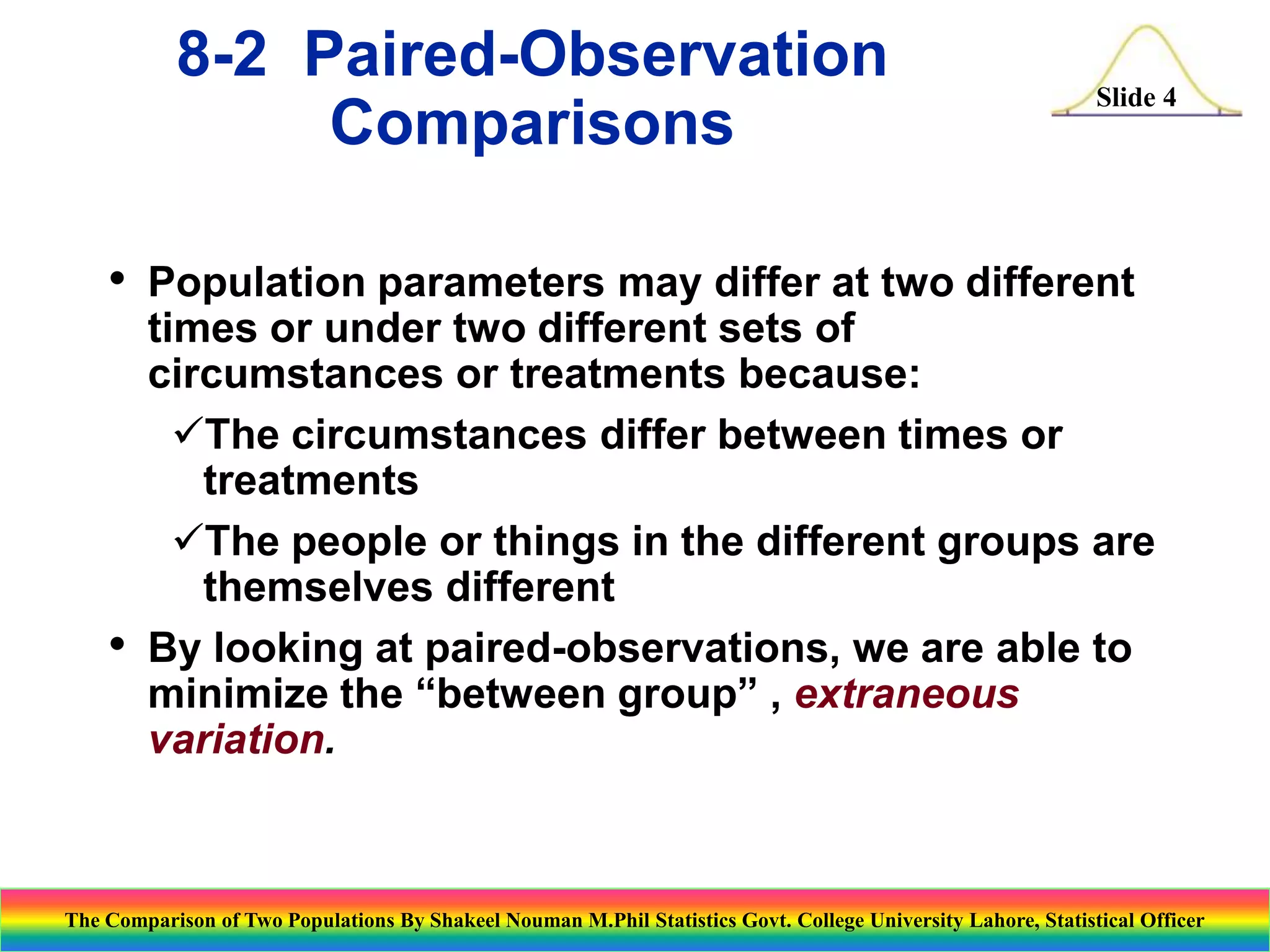
![Confidence Intervals Using the
Pooled Variance
Slide 30
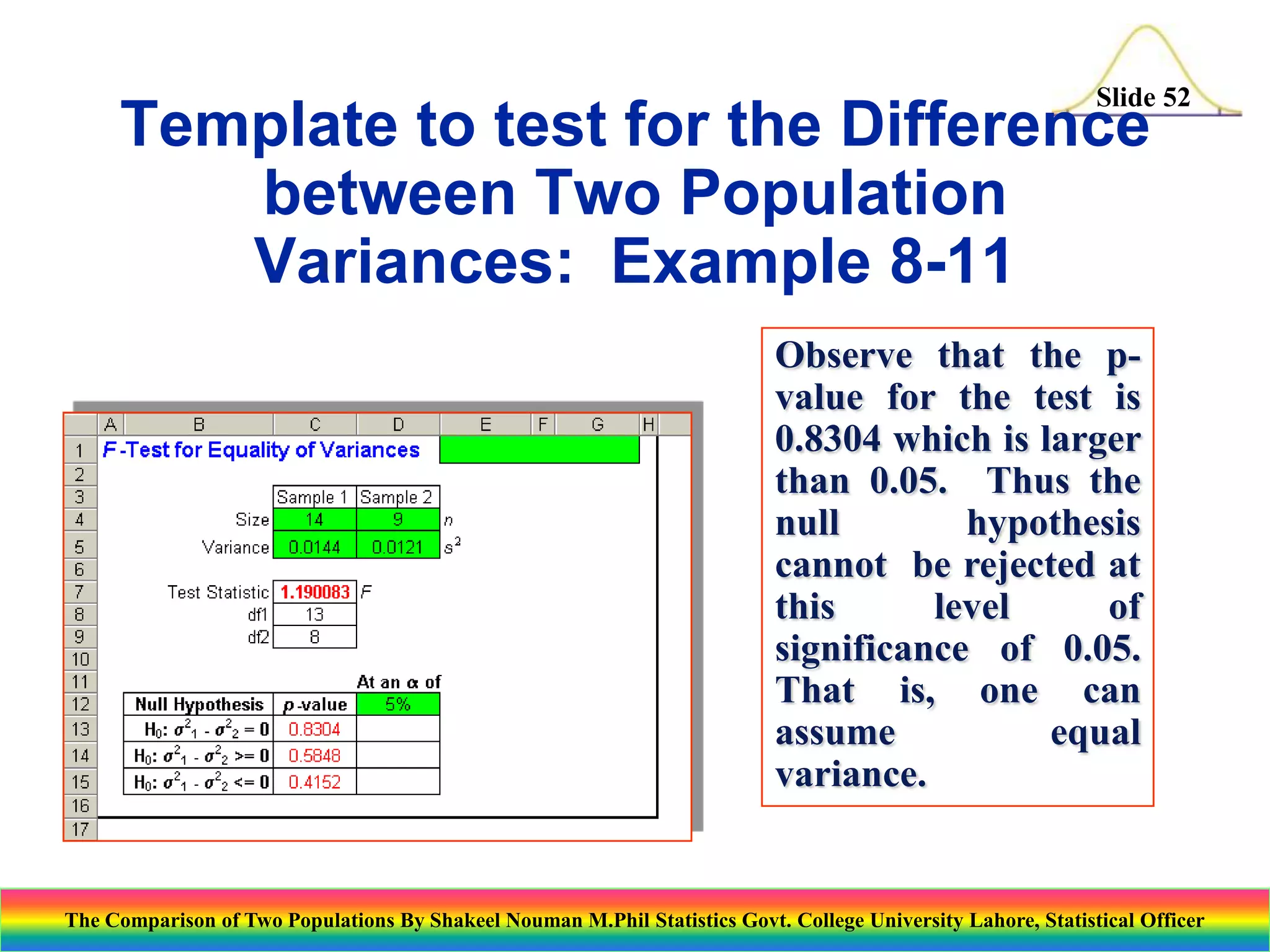
A (1-) 100% confidence interval for the difference between two
population means, 1- 2 , using independent random samples and
assuming equal population variances:
( x1 - x2 ) t
2 1
sp
n1
+
n2
1
2
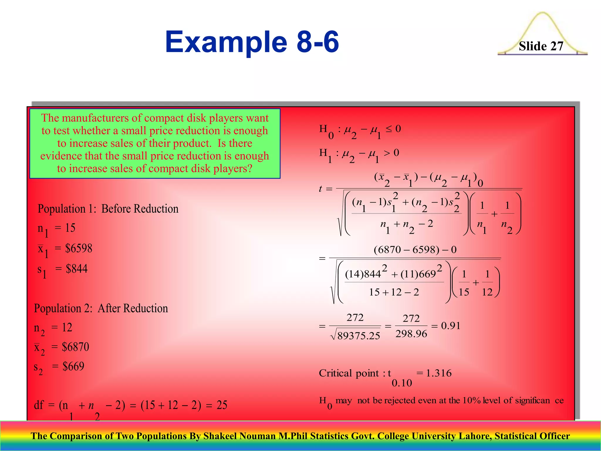
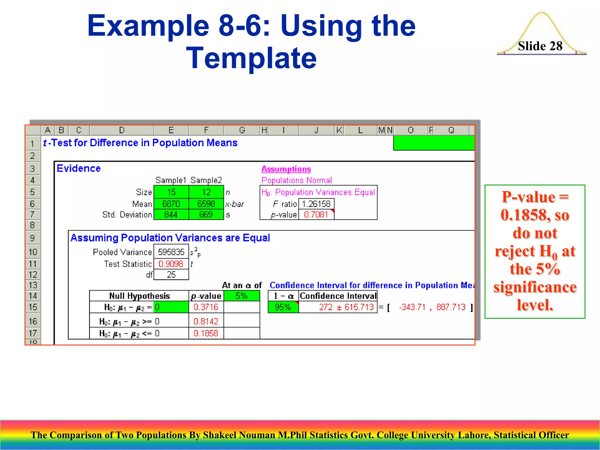
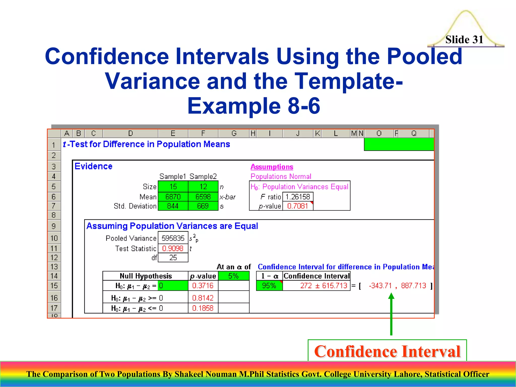
A 95% confidence interval using the data in Example 8-6:
( x1 - x 2 ) t
2
sp
1 + 1
n1 n2
( 6870 - 6598 ) 2 .06 ( 595835)( 0.15) [ -343.85,887 .85]
2
The Comparison of Two Populations By Shakeel Nouman M.Phil Statistics Govt. College University Lahore, Statistical Officer](https://image.slidesharecdn.com/thecomparisonoftwopopulations-140129013701-phpapp02/75/The-comparison-of-two-populations-30-2048.jpg)
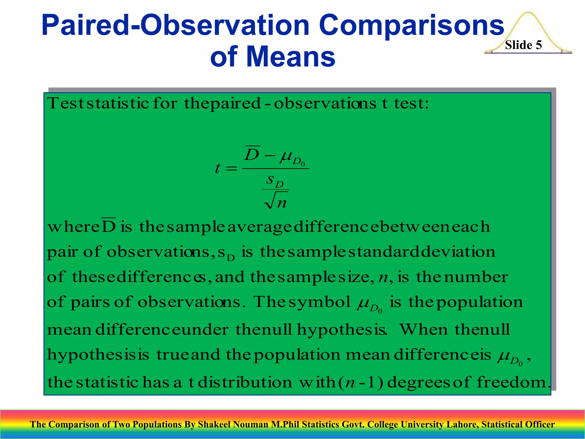
![Confidence Intervals for the
Difference between Two
Population Proportions
Slide 40
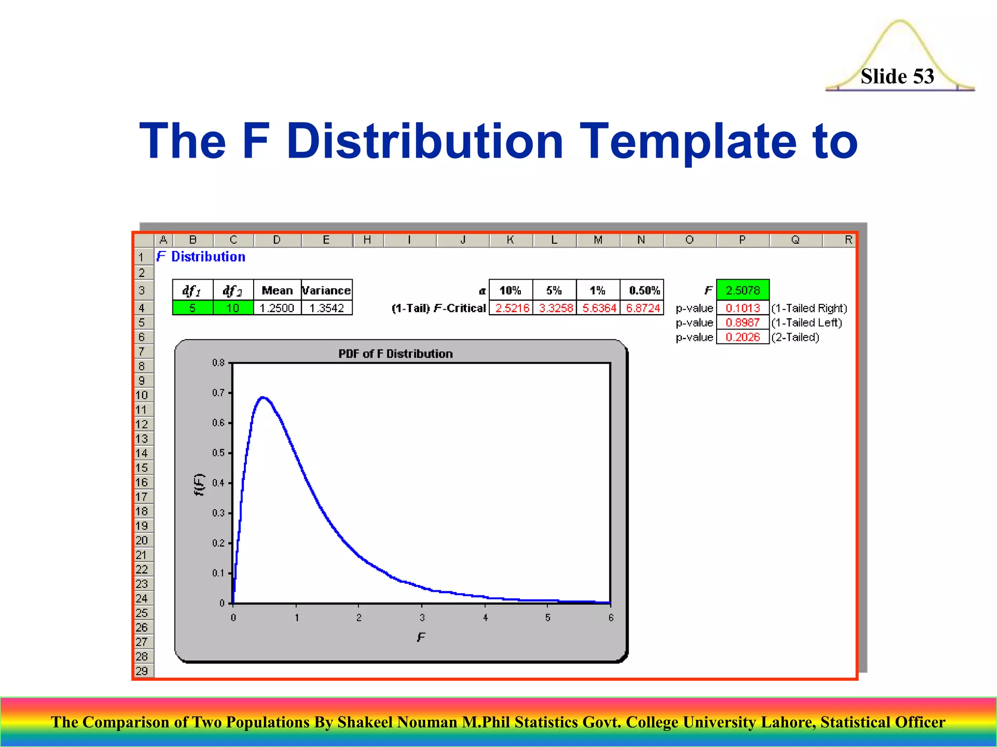
A (1- 100% large-sample confidence interval for the difference
)
between two population proportions:
( p1 - p 2 ) z
p (1 - p )
1
1
n1 +
p (1 - p )
2
2
n2
2
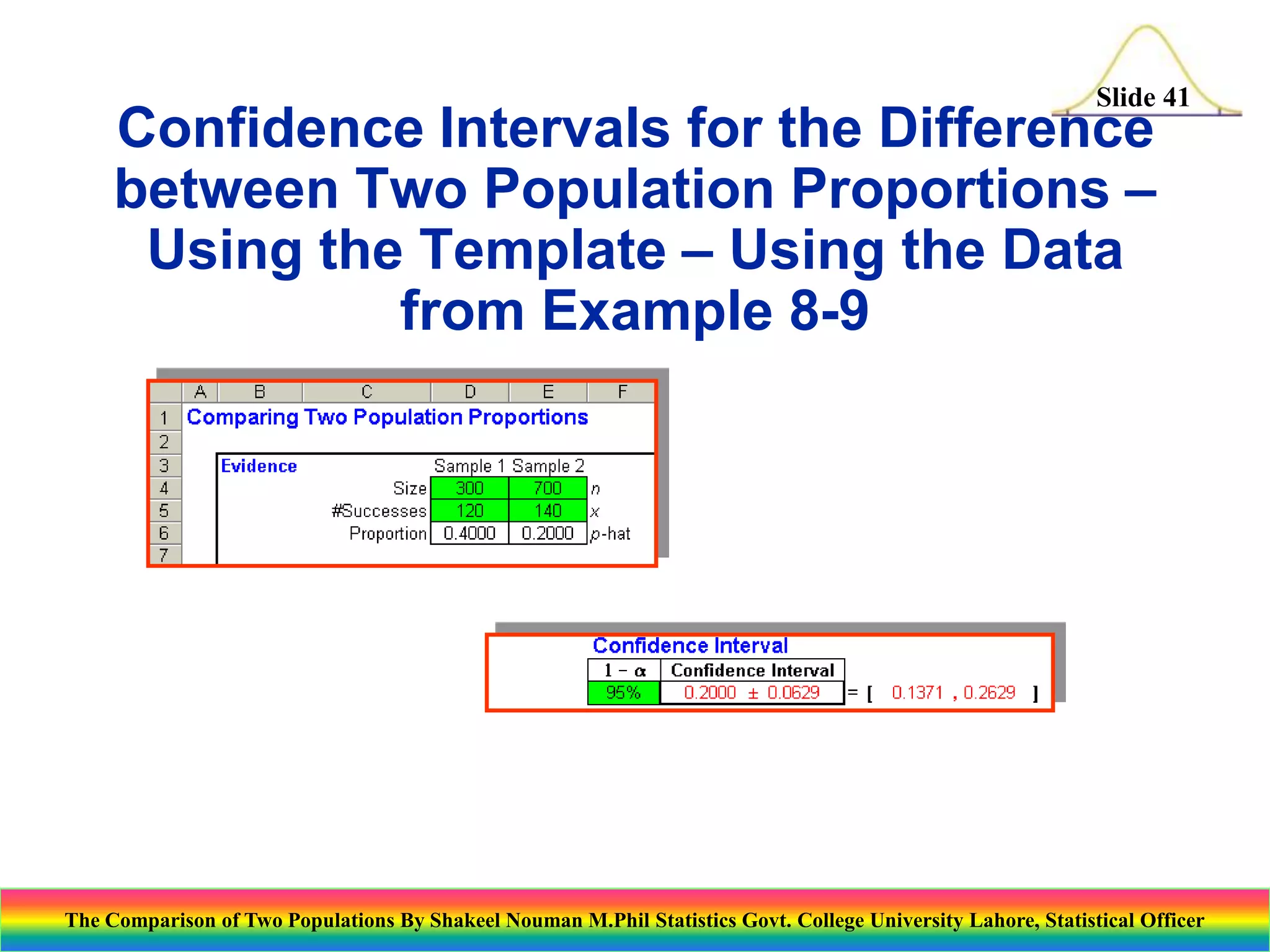
A 95% confidence interval using the data in example 8-9:
p1 (1 - p1 ) p 2 (1 - p 2 )
( 0.4 - 0.2) 1.96 ( 0.4 )( 0.6) + ( 0.2)( 0.8)
( p1 - p 2 ) z
+
n2
300
700
n1
2
0.2 (1.96)( 0.0321) 0.2 0.063 [ 0.137 ,0.263]
The Comparison of Two Populations By Shakeel Nouman M.Phil Statistics Govt. College University Lahore, Statistical Officer](https://image.slidesharecdn.com/thecomparisonoftwopopulations-140129013701-phpapp02/75/The-comparison-of-two-populations-40-2048.jpg)


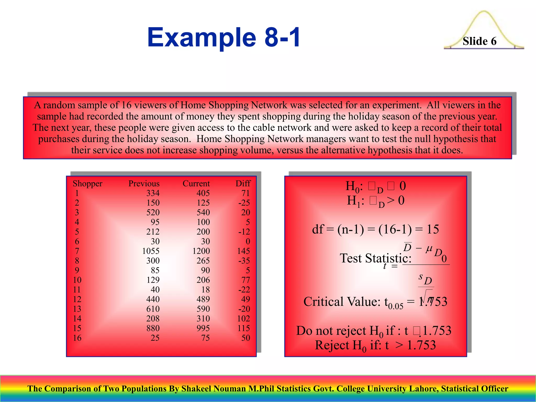
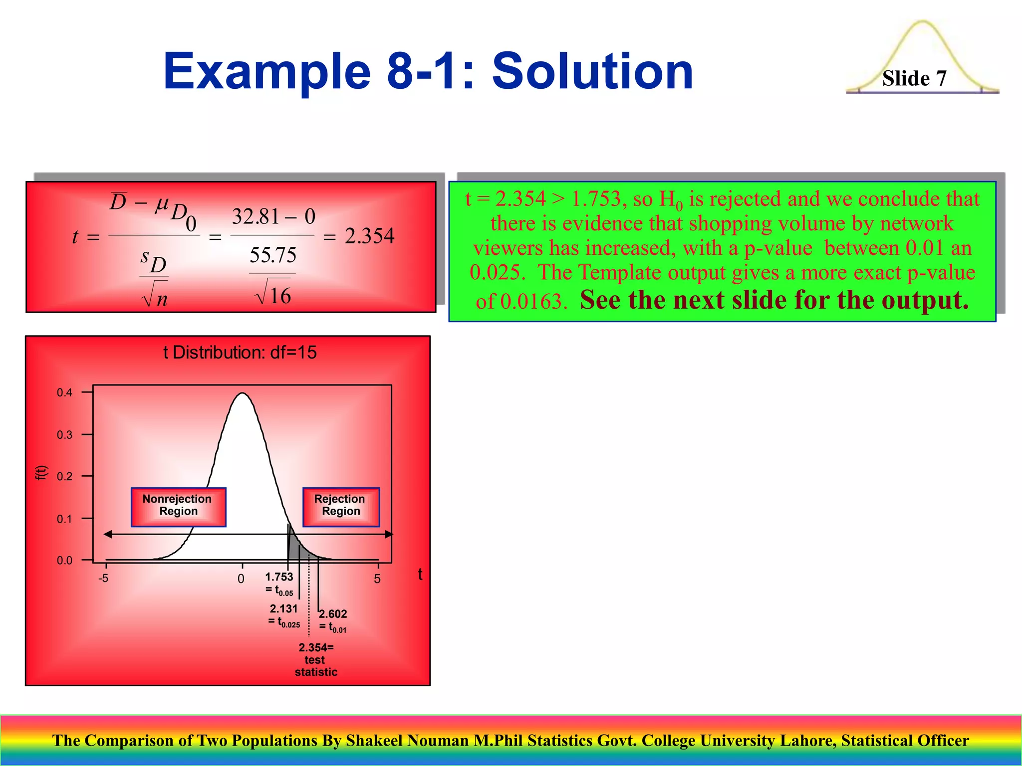
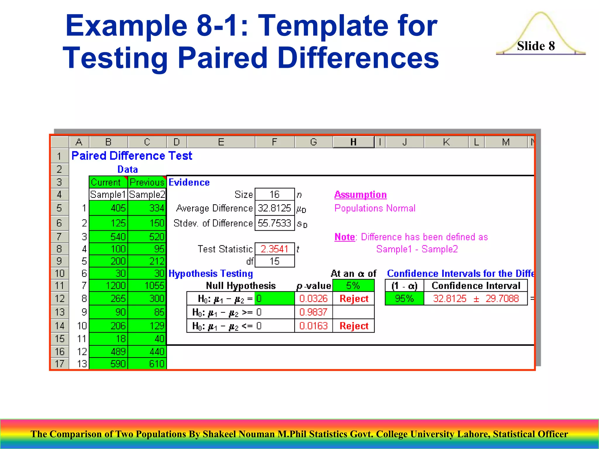
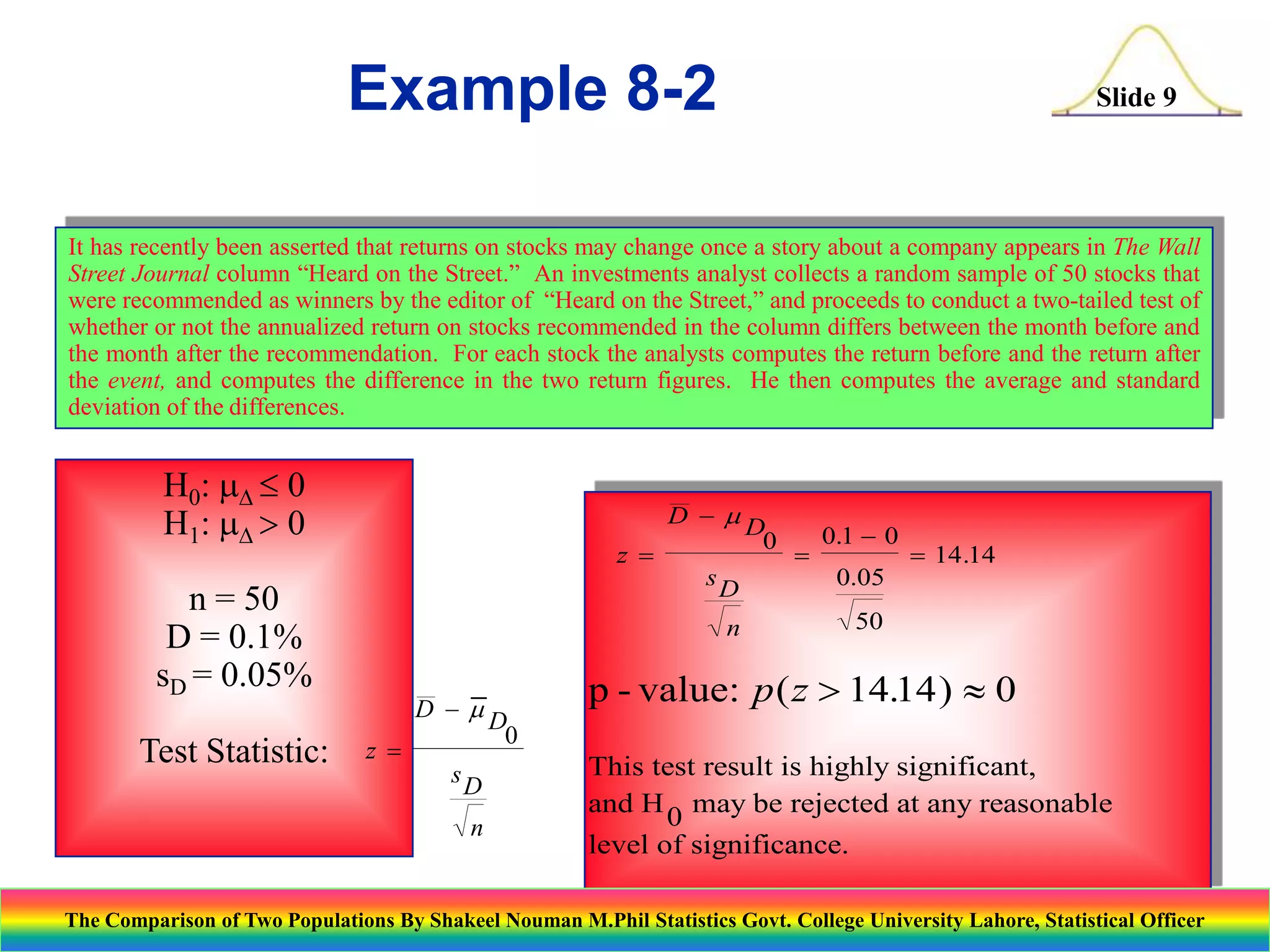
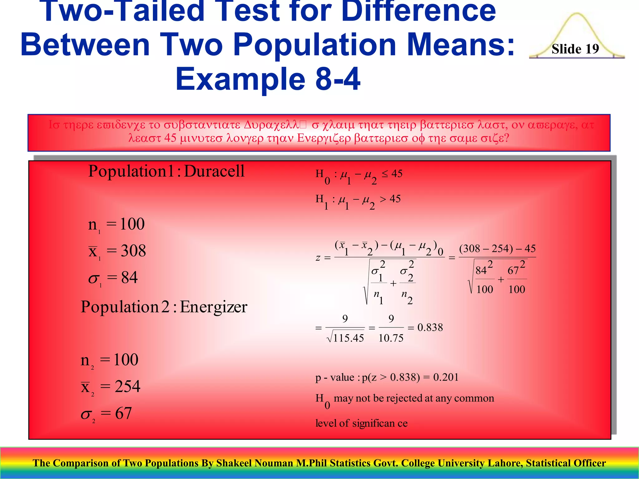
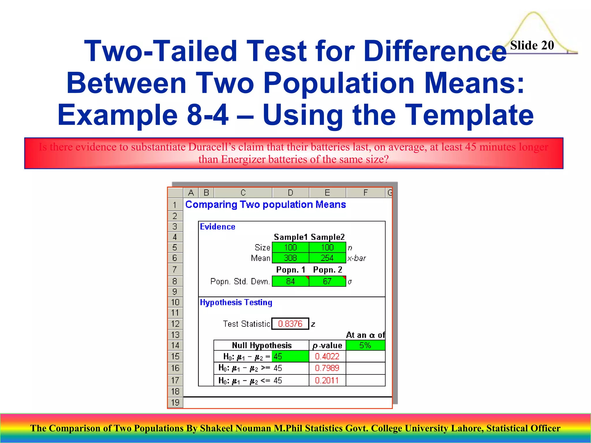
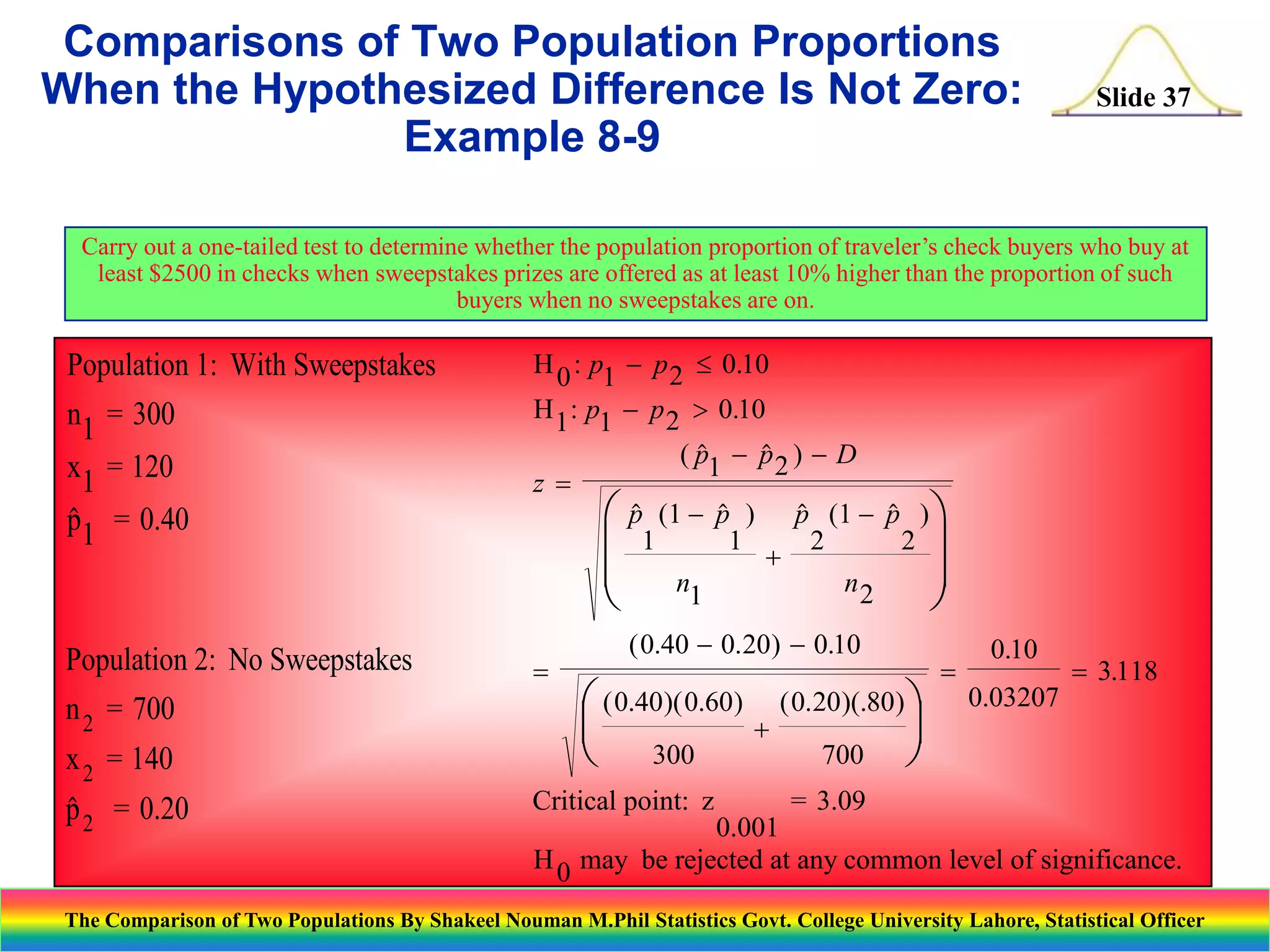
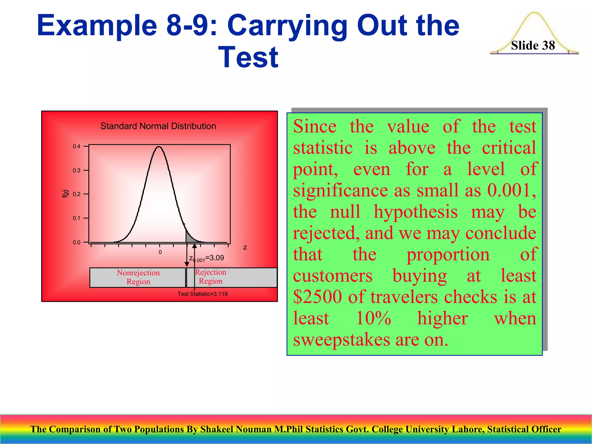
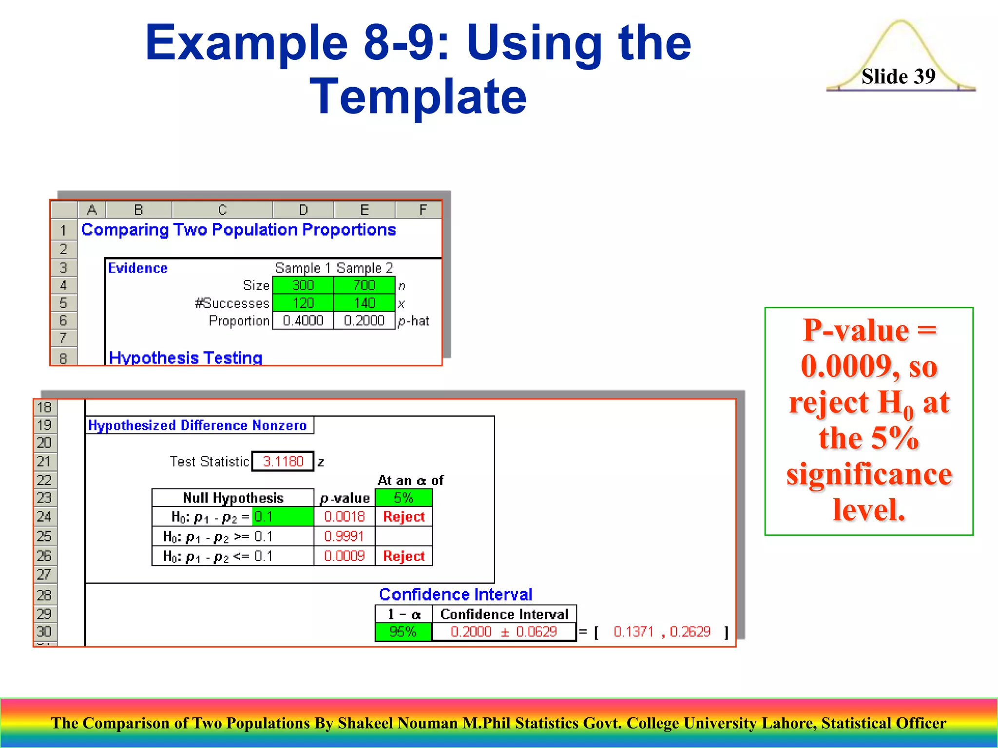
This document presents an overview of statistical techniques for comparing two populations. It discusses paired sample comparisons using a t-test and independent sample comparisons using a z-test. Examples are provided to demonstrate hypothesis testing to examine differences in population means and proportions. Specific topics covered include: paired t-tests, independent z-tests, testing situations for comparing two means, test statistics and examples comparing credit card charges and battery life. Templates are shown for conducting the tests in several examples.


