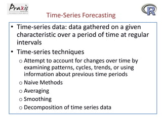
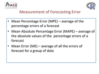
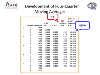
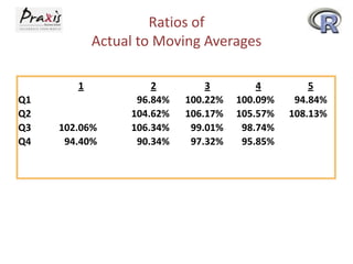
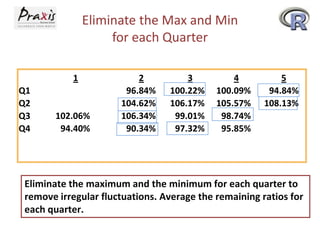
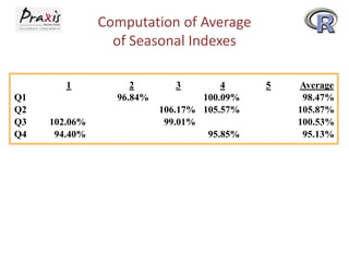
Time Series Forecasting: Objectives
• Gain a general understanding of time series forecasting
techniques.
• Understand the four possible components of time-series
data.
• Understand stationary forecasting techniques.
• Understand how to use regression models for trend analysis.
• Learn how to decompose time-series data into their various
elements and to forecast by using decomposition
techniques.
• Understand the nature of autocorrelation and how to
test for it.
• Understand auto-regression in forecasting.
Time-Series Forecasting
• Time-series data: data gathered on a given
characteristic over a period of time at regular
intervals
• Time-series techniques
o Attempt to account for changes over time by
examining patterns, cycles, trends, or using
information about previous time periods
o Naive Methods
o Averaging
o Smoothing
o Decomposition of time series data
Time Series Components
• Trend – long term general direction, typically 8 to
10 years
• Cycles (Cyclical effects) – patterns of highs and
lows through which data move over time periods
usually of more than a year, typically 3 to 5 years
• Seasonal effects – shorter cycles, which usually
occur in time periods of less than one year.
• Irregular fluctuations – rapid changes or “bleeps”
in the data, which occur in even shorter time
frames than seasonal effects.
Time-Series Effects
Time Series Components
• Stationary time-series - data that contain no trend,
cyclical, or seasonal effects.
• Error of individual forecast et – the difference
between the actual value xt and the forecast of that
value Ft i.e.
Measurement of Forecasting Error
• Error of the Individual Forecast (et = Xt – Ft) is the
difference between the actual value xt and the forecast of
that value Ft.
• Mean Absolute Deviation (MAD) - is the mean, or
average, of the absolute values of the errors.
• Mean Square Error (MSE) - circumvents the problem
of the canceling effects of positive and negative forecast
errors.
– Computed by squaring each error and averaging the
squared errors.
Measurement of Forecasting Error
• Mean Percentage Error (MPE) – average of the
percentage errors of a forecast
• Mean Absolute Percentage Error (MAPE) – average of
the absolute values of the percentage errors of a
forecast
• Mean Error (ME) – average of all the errors of
forecast for a group of data
Nonfarm Partnership Tax Returns:
Actual and Forecast with = .7
Year Actual Forecast Error
1 1402
2 1458 1402.0 56.0
3 1553 1441.2 111.8
4 1613 1519.5 93.5
5 1676 1584.9 91.1
6 1755 1648.7 106.3
7 1807 1723.1 83.9
8 1824 1781.8 42.2
9 1826 1811.3 14.7
10 1780 1821.6 -41.6
11 1759 1792.5 -33.5
Mean Absolute Deviation (MAD):
Nonfarm Partnership Forecasted Data
Year Actual Forecast Error |Error|
1 1402.0
2 1458.0 1402.0 56.0 56.0
3 1553.0 1441.2 111.8 111.8
4 1613.0 1519.5 93.5 93.5
5 1676.0 1584.9 91.1 91.1
6 1755.0 1648.7 106.3 106.3
7 1807.0 1723.1 83.9 83.9
8 1824.0 1781.8 42.2 42.2
9 1826.0 1811.3 14.7 14.7
10 1780.0 1821.6 -41.6 41.6
11 1759.0 1792.5 -33.5 33.5
674.5
Mean Square Error (MSE):
Nonfarm Partnership Forecasted Data
Year Actual Forecast Error Error2
1 1402
2 1458 1402.0 56.0
3 1553 1441.2 111.8
4 1613 1519.5 93.5
5 1676 1584.9 91.1
6 1755 1648.7 106.3
7 1807 1723.1 83.9
8 1824 1781.8 42.2
9 1826 1811.3 14.7
10 1780 1821.6 -41.6
11 1759 1792.5 -33.5
55864.2
3136.0
12499.2
8749.7
8292.3
11303.6
7038.5
1778.2
214.6
1731.0
1121.0
Smoothing Techniques
• Smoothing techniques produce forecasts based on
“smoothing out” the irregular fluctuation effects in
the time-series data
• Naive Forecasting Models - simple models in which
it is assumed that the more recent time periods of
data represent the best predictions or forecasts for
future outcomes
Smoothing Techniques
• Averaging Models - the forecast for time period
t is the average of the values for a given number of
previous time periods:
o Simple Averages
o Moving Averages
o Weighted Moving Averages
• Exponential Smoothing - is used to weight data
from previous time periods with exponentially
decreasing importance in the forecast.
Simple Average Model
The forecast for time
period t is the average of
the values for a given
number of previous time
periods.
Month Year
Cents
per
Gallon Month Year
Cents
per
Gallon
January 2 61.3 January 3 58.2
February 63.3 February 58.3
March 62.1 March 57.7
April 59.8 April 56.7
May 58.4 May 56.8
June 57.6 June 55.5
July 55.7 July 53.8
August 55.1 August 52.8
September 55.7 September
October 56.7 October
November 57.2 November
December 58.0 December
The monthly average last
12 months was 56.45,
so I predict
56.45 for September.
Moving Average
• Updated (recomputed) for every new time period
• May be difficult to choose optimal number of periods
• May not adjust for trend, cyclical, or seasonal effects
Update each period.
Demonstration Problem 15.1:
Four-Month Moving Average
Shown in the following table here are shipments
(in millions of dollars) for electric lighting and wiring
equipment over a 12-month period. Use these data
to compute a 4-month moving average for all
available months.
Demonstration Problem 15.1:
Four-Month Moving Average
Months Shipments
4-Mo
Moving
Average
Forecast
Error
January 1056
February 1345
March 1381
April 1191
May 1259 1243.25 15.75
June 1361 1294.00 67.00
July 1110 1298.00 -188.00
August 1334 1230.25 103.75
September 1416 1266.00 150.00
October 1282 1305.25 -23.25
November 1341 1285.50 55.50
December 1382 1343.25 38.75
Demonstration Problem 15.1:
Four-Month Moving Average
Weighted Moving Average
Forecasting Model
A moving average in which some time periods are
weighted differently than others.
Example of 3 months
Weighted average
where last month’s value
value for the previous month
value for the month before the
previous month
The denominator = the total of weights
1tM
2tM
3tM
Demonstration Problem 15.2:
Four-Month Weighted Moving Average
Months Shipments
4-Month
Weighted
Moving
Average
Forecast
Error
January 1056
February 1345
March 1381
April 1191
May 1259 1240.88 18.13
June 1361 1268.00 93.00
July 1110 1316.75 -206.75
August 1334 1201.50 132.50
September 1416 1272.00 144.00
October 1282 1350.38 -68.38
November 1341 1300.50 40.50
December 1382 1334.75 47.25
Exponential Smoothing
Used to weight data from previous time periods with
exponentially decreasing importance in the forecast
t t t
t
t
t
F X F
F
F
X
where
1
1
1
: the forecast for the next time period (t+1)
the forecast for the present time period (t)
the actual value for the present time period
= a value between 0 and 1
is the exponential
smoothing constant
Demonstration Problem 15.3: = 0.2
The U.S. Census Bureau reports the total units of new
privately owned housing started over a 16-year recent
period in the United States are given here. Use
exponential smoothing to forecast the values for each
ensuing time period. Work the problem using = 0.2,
0.5, and 0.8
Demonstration Problem 15.3: = 0.2
= 0.2
Year
Housing Units
(1,000) F e |e| e2
1990 1193 -- -- -- --
1991 1014 1193.0 -179 179 32041
1992 1200 1157.2 42.8 42.8 1832
1993 1288 1165.8 122.2 122.2 14933
1994 1457 1190.2 266.8 266.8 71182
1995 1354 1243.6 110.4 110.4 12188
1996 1477 1265.7 211.3 211.3 44648
1997 1474 1307.9 166.1 166.1 27589
1998 1617 1341.1 275.9 275.9 76121
1999 1641 1396.3 244.7 244.7 59878
2000 1569 1445.2 123.8 123.8 15326
2001 1603 1470.0 133.0 133.0 17689
2002 1705 1496.6 208.4 208.4 43431
2003 1848 1538.3 309.7 309.7 95914
2004 1956 1600.2 355.8 355.8 126594
2005 2068 1671.4 396.6 396.6 157292
3146.5 796657
MAD 209.8
MSE 53110
Demonstration Problem 15.3: = 0.8
= 0.8
Year
Housing Units
(1,000) F e |e| e2
1990 1193 -- -- -- --
1991 1014 1193.0 -179 179 64.0
1992 1200 1049.8 150.2 150.2 3770.0
1993 1288 1170.0 118.0 118.0 29832.2
1994 1457 1264.4 192.6 192.6 27736.9
1995 1354 1418.5 -64.5 64.5 21114.6
1996 1477 1366.9 110.1 110.1 44970.2
1997 1474 1455.0 19.0 19.0 49023.4
1998 1617 1470.2 146.8 146.8 20083.9
1999 1641 1587.6 53.4 53.4 13535.8
2000 1569 1630.3 -61.3 61.3 36967.3
2001 1603 1581.3 21.7 21.7 4166.2
2002 1705 1598.7 106.3 106.3 12120.0
2003 1848 1683.7 164.3 164.3 361.7
2004 1956 1815.1 140.9 140.9 21551.3
2005 2068 1927.8 140.2 140.2 6140.4
1668.3 228896
MAD 111.2
MSE 15245.9
Trend Analysis
• Trend – long run general direction of climate over
an extended time
• Linear Trend
• Quadratic Trend
• Holt’s Two Parameter Exponential Smoothing -
Holt’s technique uses weights (β) to smooth the
trend in a manner similar to the smoothing used in
single exponential smoothing (α)
Average Hours Worked per Week
by Canadian Manufacturing Workers
Following table provides the data needed to
compute a quadratic regression trend model on
the manufacturing workweek data
Average Hours Worked per Week
by Canadian Manufacturing Workers
Period Hours Period Hours Period Hours Period Hours
1 37.2 11 36.9 21 35.6 31 35.7
2 37.0 12 36.7 22 35.2 32 35.5
3 37.4 13 36.7 23 34.8 33 35.6
4 37.5 14 36.5 24 35.3 34 36.3
5 37.7 15 36.3 25 35.6 35 36.5
6 37.7 16 35.9 26 35.6
7 37.4 17 35.8 27 35.6
8 37.2 18 35.9 28 35.9
9 37.3 19 36.0 29 36.0
10 37.2 20 35.7 30 35.7
Excel Regression Output using
Linear Trend
Regression Statistics
Multiple R
R Square
Adjusted R Square
Standard Error
Observations
ANOVA
SS MS F Significance F
Regression 1 13.4467 13.4467 51.91 .00000003
Residual 33 8.5487 0.2591
Total 34 21.9954
Coefficients Standard Error t Stat P-value
Intercept 37.4161 0.17582 212.81 .0000000
Period -0.0614 0.00852 -7.20 .00000003
i ti i
t
Y X
X
where
Y
0 1
37 416 0 0614
:
 . .
data value for period i
time period
i
i
Y
X
35
0.782
0.611
0.5600
0.509
df
Excel Regression Output using
Quadratic Trend
Regression Statistics
Multiple R 0.8723
R Square 0.761
Adjusted R Square 0.747
Standard Error 0.405
Observations 35
ANOVA
df SS MS F Significance F
Regression 2 16.7483 8.3741 51.07 1.10021E-10
Residual 32 5.2472 0.1640
Total 34 21.9954
Coefficients Standard Error t Stat P-value
Intercept 38.16442 0.21766 175.34 2.61E-49
Period -0.18272 0.02788 -6.55 2.21E-07
Period2 0.00337 0.00075 4.49 8.76E-05
i ti ti i
ti
t t
Y X X
X
X X
where
Y
0 1 2
2
2
2
38164 0183 0 003
:
 . . .
data value for period i
time period
the square of the i period
i
i
th
Y
X
Graph of Canadian Workweek Data
with a Second-Degree Polynomial Fit
Demonstration Problem 15.4
Data on the employed U.S. civilian labour force (in
100,000) for 1991 through 2008, obtained from the U.S.
Bureau of Labor Statistics. Use regression analysis to fit
a trend line through the data and explore a quadratic
trend. Compare the models.
Regression Output from Package
Model Comparison
Linear
Model
Quadratic
Model
Time Series: Decomposition
Decomposition – Breaking down the effects of
time series data into four component parts:
trend, cyclical, seasonal, and irregular
Basis for analysis is the Multiplicative Model
Y = T · C · S · I
where:
T = trend component
C = cyclical component
S = seasonal component
I = irregular component
Household Appliance Shipment Data
Illustration of decomposition process: the 5-year quarterly
time-series data on U.S. shipments of household appliances
Year Quarter Shipments Year Quarter Shipments
1 1 4009 4 1 4595
2 4321 2 4799
3 4224 3 4417
4 3944 4 4258
2 1 4123 5 1 4245
2 4522 2 4900
3 4657 3 4585
4 4030 4 4533
3 1 4493
2 4806
3 4551
4 4485
Shipments in $1,000,000.
Development of Four-Quarter
Moving Averages
Quarter Shipments
4 Qtr
M.T. 2 Yr M.T.
4 Qtr
Centered
M.A.
Ratios of
Actual
Values to
M.A.
1 1 4009
2 4321 16,498
3 4224 16,612 33,110 4139 102.06%
4 3944 16,813 33,425 4178 94.40%
2 1 4123 17,246 34,059 4257 96.84%
2 4522 17,332 34,578 4322 104.62%
3 4657 17,702 35,034 4379 106.34%
4 4030 17,986 35,688 4461 90.34%
3 1 4493 17,880 35,866 4483 100.22%
2 4806 18,335 36,215 4527 106.17%
3 4551 18,437 36,772 4597 99.01%
4 4485 18,430 36,867 4608 97.32%
4 1 4595 18,296 36,726 4591 100.09%
2 4799 18,069 36,365 4546 105.57%
3 4417 17,719 35,788 4474 98.74%
4 4258 17,820 35,539 4442 95.85%
5 1 4245 17,988 35,808 4476 94.84%
2 4900 18,263 36,251 4531 108.13%
3 4585
4 4533
S·I(100)
T·C
Ratios of
Actual to Moving Averages
1 2 3 4 5
Q1 96.84% 100.22% 100.09% 94.84%
Q2 104.62% 106.17% 105.57% 108.13%
Q3 102.06% 106.34% 99.01% 98.74%
Q4 94.40% 90.34% 97.32% 95.85%
Eliminate the Max and Min
for each Quarter
1 2 3 4 5
Q1 96.84% 100.22% 100.09% 94.84%
Q2 104.62% 106.17% 105.57% 108.13%
Q3 102.06% 106.34% 99.01% 98.74%
Q4 94.40% 90.34% 97.32% 95.85%
Eliminate the maximum and the minimum for each quarter to
remove irregular fluctuations. Average the remaining ratios for
each quarter.
Computation of Average
of Seasonal Indexes
1 2 3 4 5 Average
Q1 96.84% 100.09% 98.47%
Q2 106.17% 105.57% 105.87%
Q3 102.06% 99.01% 100.53%
Q4 94.40% 95.85% 95.13%
Deseasonalized
House Appliance Data
Year Quarter
Shipments
(T*C*S*I)
Seasonal
Indexes
(S)
Deseasonalized
Data
(T*C*I)
1 1 4009 98.47% 4,071
2 4321 105.87% 4,081
3 4224 100.53% 4,202
4 3944 95.12% 4,146
2 1 4123 98.47% 4,187
2 4522 105.87% 4,271
3 4657 100.53% 4,632
4 4030 95.12% 4,237
3 1 4493 98.47% 4,563
2 4806 105.87% 4,540
3 4551 100.53% 4,527
4 4485 95.12% 4,715
4 1 4595 98.47% 4,666
2 4799 105.87% 4,533
3 4417 100.53% 4,393
4 4258 95.12% 4,476
5 1 4245 98.47% 4,311
2 4900 105.87% 4,628
3 4585 100.53% 4,561
4 4533 95.12% 4,765
Autocorrelation (Serial Correlation)
• Autocorrelation occurs in data when the error terms of
a regression forecasting model are correlated and not
independent, particularly with economic variables.
• Potential Problems
• Estimates of the regression coefficients no longer have
the minimum variance property and may be inefficient.
• The variance of the error terms may be greatly
underestimated by the mean square error value.
• The true standard deviation of the estimated regression
coefficient may be seriously underestimated.
• The confidence intervals and tests using the t and F
distributions are no longer strictly applicable.
Autocorrelation (Serial Correlation)
Durbin-Watson Test
H
Ha
0 0
0
:
:
D
t t
where
e e
e
t
n
t
t
n
2
2
2
1
1
: n = the number of observations
If D > do not reject H (there is no significant autocorrelation).
If D < , reject H (there is significant autocorrelation).
If , the test is inconclusive.
U
0
L
0
L U
d
d
d d
,
D
Autoregression Model
Overcoming Autocorrelation Problem
• Addition of Independent Variables
• Transforming Variables
 First-differences approach - Often autocorrelation occurs
in regression analyses when one or more predictor
variables have been left out of the analysis
 Percentage change from period to period - each value of x
is subtracted from each succeeding time period value of x;
these “differences” become the new and transformed x
variable, the same for y
 Use autoregression - multiple regression technique in
which the independent variables are time-lagged versions
of the dependent variable

Statr session 25 and 26

  • 1.
    Time Series Forecasting:Objectives • Gain a general understanding of time series forecasting techniques. • Understand the four possible components of time-series data. • Understand stationary forecasting techniques. • Understand how to use regression models for trend analysis. • Learn how to decompose time-series data into their various elements and to forecast by using decomposition techniques. • Understand the nature of autocorrelation and how to test for it. • Understand auto-regression in forecasting.
  • 2.
    Time-Series Forecasting • Time-seriesdata: data gathered on a given characteristic over a period of time at regular intervals • Time-series techniques o Attempt to account for changes over time by examining patterns, cycles, trends, or using information about previous time periods o Naive Methods o Averaging o Smoothing o Decomposition of time series data
  • 3.
    Time Series Components •Trend – long term general direction, typically 8 to 10 years • Cycles (Cyclical effects) – patterns of highs and lows through which data move over time periods usually of more than a year, typically 3 to 5 years • Seasonal effects – shorter cycles, which usually occur in time periods of less than one year. • Irregular fluctuations – rapid changes or “bleeps” in the data, which occur in even shorter time frames than seasonal effects.
  • 4.
  • 5.
    Time Series Components •Stationary time-series - data that contain no trend, cyclical, or seasonal effects. • Error of individual forecast et – the difference between the actual value xt and the forecast of that value Ft i.e.
  • 6.
    Measurement of ForecastingError • Error of the Individual Forecast (et = Xt – Ft) is the difference between the actual value xt and the forecast of that value Ft. • Mean Absolute Deviation (MAD) - is the mean, or average, of the absolute values of the errors. • Mean Square Error (MSE) - circumvents the problem of the canceling effects of positive and negative forecast errors. – Computed by squaring each error and averaging the squared errors.
  • 7.
    Measurement of ForecastingError • Mean Percentage Error (MPE) – average of the percentage errors of a forecast • Mean Absolute Percentage Error (MAPE) – average of the absolute values of the percentage errors of a forecast • Mean Error (ME) – average of all the errors of forecast for a group of data
  • 8.
    Nonfarm Partnership TaxReturns: Actual and Forecast with = .7 Year Actual Forecast Error 1 1402 2 1458 1402.0 56.0 3 1553 1441.2 111.8 4 1613 1519.5 93.5 5 1676 1584.9 91.1 6 1755 1648.7 106.3 7 1807 1723.1 83.9 8 1824 1781.8 42.2 9 1826 1811.3 14.7 10 1780 1821.6 -41.6 11 1759 1792.5 -33.5
  • 9.
    Mean Absolute Deviation(MAD): Nonfarm Partnership Forecasted Data Year Actual Forecast Error |Error| 1 1402.0 2 1458.0 1402.0 56.0 56.0 3 1553.0 1441.2 111.8 111.8 4 1613.0 1519.5 93.5 93.5 5 1676.0 1584.9 91.1 91.1 6 1755.0 1648.7 106.3 106.3 7 1807.0 1723.1 83.9 83.9 8 1824.0 1781.8 42.2 42.2 9 1826.0 1811.3 14.7 14.7 10 1780.0 1821.6 -41.6 41.6 11 1759.0 1792.5 -33.5 33.5 674.5
  • 10.
    Mean Square Error(MSE): Nonfarm Partnership Forecasted Data Year Actual Forecast Error Error2 1 1402 2 1458 1402.0 56.0 3 1553 1441.2 111.8 4 1613 1519.5 93.5 5 1676 1584.9 91.1 6 1755 1648.7 106.3 7 1807 1723.1 83.9 8 1824 1781.8 42.2 9 1826 1811.3 14.7 10 1780 1821.6 -41.6 11 1759 1792.5 -33.5 55864.2 3136.0 12499.2 8749.7 8292.3 11303.6 7038.5 1778.2 214.6 1731.0 1121.0
  • 11.
    Smoothing Techniques • Smoothingtechniques produce forecasts based on “smoothing out” the irregular fluctuation effects in the time-series data • Naive Forecasting Models - simple models in which it is assumed that the more recent time periods of data represent the best predictions or forecasts for future outcomes
  • 12.
    Smoothing Techniques • AveragingModels - the forecast for time period t is the average of the values for a given number of previous time periods: o Simple Averages o Moving Averages o Weighted Moving Averages • Exponential Smoothing - is used to weight data from previous time periods with exponentially decreasing importance in the forecast.
  • 13.
    Simple Average Model Theforecast for time period t is the average of the values for a given number of previous time periods. Month Year Cents per Gallon Month Year Cents per Gallon January 2 61.3 January 3 58.2 February 63.3 February 58.3 March 62.1 March 57.7 April 59.8 April 56.7 May 58.4 May 56.8 June 57.6 June 55.5 July 55.7 July 53.8 August 55.1 August 52.8 September 55.7 September October 56.7 October November 57.2 November December 58.0 December The monthly average last 12 months was 56.45, so I predict 56.45 for September.
  • 14.
    Moving Average • Updated(recomputed) for every new time period • May be difficult to choose optimal number of periods • May not adjust for trend, cyclical, or seasonal effects Update each period.
  • 15.
    Demonstration Problem 15.1: Four-MonthMoving Average Shown in the following table here are shipments (in millions of dollars) for electric lighting and wiring equipment over a 12-month period. Use these data to compute a 4-month moving average for all available months.
  • 16.
    Demonstration Problem 15.1: Four-MonthMoving Average Months Shipments 4-Mo Moving Average Forecast Error January 1056 February 1345 March 1381 April 1191 May 1259 1243.25 15.75 June 1361 1294.00 67.00 July 1110 1298.00 -188.00 August 1334 1230.25 103.75 September 1416 1266.00 150.00 October 1282 1305.25 -23.25 November 1341 1285.50 55.50 December 1382 1343.25 38.75
  • 17.
  • 18.
    Weighted Moving Average ForecastingModel A moving average in which some time periods are weighted differently than others. Example of 3 months Weighted average where last month’s value value for the previous month value for the month before the previous month The denominator = the total of weights 1tM 2tM 3tM
  • 19.
    Demonstration Problem 15.2: Four-MonthWeighted Moving Average Months Shipments 4-Month Weighted Moving Average Forecast Error January 1056 February 1345 March 1381 April 1191 May 1259 1240.88 18.13 June 1361 1268.00 93.00 July 1110 1316.75 -206.75 August 1334 1201.50 132.50 September 1416 1272.00 144.00 October 1282 1350.38 -68.38 November 1341 1300.50 40.50 December 1382 1334.75 47.25
  • 20.
    Exponential Smoothing Used toweight data from previous time periods with exponentially decreasing importance in the forecast t t t t t t F X F F F X where 1 1 1 : the forecast for the next time period (t+1) the forecast for the present time period (t) the actual value for the present time period = a value between 0 and 1 is the exponential smoothing constant
  • 21.
    Demonstration Problem 15.3:= 0.2 The U.S. Census Bureau reports the total units of new privately owned housing started over a 16-year recent period in the United States are given here. Use exponential smoothing to forecast the values for each ensuing time period. Work the problem using = 0.2, 0.5, and 0.8
  • 22.
    Demonstration Problem 15.3:= 0.2 = 0.2 Year Housing Units (1,000) F e |e| e2 1990 1193 -- -- -- -- 1991 1014 1193.0 -179 179 32041 1992 1200 1157.2 42.8 42.8 1832 1993 1288 1165.8 122.2 122.2 14933 1994 1457 1190.2 266.8 266.8 71182 1995 1354 1243.6 110.4 110.4 12188 1996 1477 1265.7 211.3 211.3 44648 1997 1474 1307.9 166.1 166.1 27589 1998 1617 1341.1 275.9 275.9 76121 1999 1641 1396.3 244.7 244.7 59878 2000 1569 1445.2 123.8 123.8 15326 2001 1603 1470.0 133.0 133.0 17689 2002 1705 1496.6 208.4 208.4 43431 2003 1848 1538.3 309.7 309.7 95914 2004 1956 1600.2 355.8 355.8 126594 2005 2068 1671.4 396.6 396.6 157292 3146.5 796657 MAD 209.8 MSE 53110
  • 23.
    Demonstration Problem 15.3:= 0.8 = 0.8 Year Housing Units (1,000) F e |e| e2 1990 1193 -- -- -- -- 1991 1014 1193.0 -179 179 64.0 1992 1200 1049.8 150.2 150.2 3770.0 1993 1288 1170.0 118.0 118.0 29832.2 1994 1457 1264.4 192.6 192.6 27736.9 1995 1354 1418.5 -64.5 64.5 21114.6 1996 1477 1366.9 110.1 110.1 44970.2 1997 1474 1455.0 19.0 19.0 49023.4 1998 1617 1470.2 146.8 146.8 20083.9 1999 1641 1587.6 53.4 53.4 13535.8 2000 1569 1630.3 -61.3 61.3 36967.3 2001 1603 1581.3 21.7 21.7 4166.2 2002 1705 1598.7 106.3 106.3 12120.0 2003 1848 1683.7 164.3 164.3 361.7 2004 1956 1815.1 140.9 140.9 21551.3 2005 2068 1927.8 140.2 140.2 6140.4 1668.3 228896 MAD 111.2 MSE 15245.9
  • 24.
    Trend Analysis • Trend– long run general direction of climate over an extended time • Linear Trend • Quadratic Trend • Holt’s Two Parameter Exponential Smoothing - Holt’s technique uses weights (β) to smooth the trend in a manner similar to the smoothing used in single exponential smoothing (α)
  • 25.
    Average Hours Workedper Week by Canadian Manufacturing Workers Following table provides the data needed to compute a quadratic regression trend model on the manufacturing workweek data
  • 26.
    Average Hours Workedper Week by Canadian Manufacturing Workers Period Hours Period Hours Period Hours Period Hours 1 37.2 11 36.9 21 35.6 31 35.7 2 37.0 12 36.7 22 35.2 32 35.5 3 37.4 13 36.7 23 34.8 33 35.6 4 37.5 14 36.5 24 35.3 34 36.3 5 37.7 15 36.3 25 35.6 35 36.5 6 37.7 16 35.9 26 35.6 7 37.4 17 35.8 27 35.6 8 37.2 18 35.9 28 35.9 9 37.3 19 36.0 29 36.0 10 37.2 20 35.7 30 35.7
  • 27.
    Excel Regression Outputusing Linear Trend Regression Statistics Multiple R R Square Adjusted R Square Standard Error Observations ANOVA SS MS F Significance F Regression 1 13.4467 13.4467 51.91 .00000003 Residual 33 8.5487 0.2591 Total 34 21.9954 Coefficients Standard Error t Stat P-value Intercept 37.4161 0.17582 212.81 .0000000 Period -0.0614 0.00852 -7.20 .00000003 i ti i t Y X X where Y 0 1 37 416 0 0614 :  . . data value for period i time period i i Y X 35 0.782 0.611 0.5600 0.509 df
  • 28.
    Excel Regression Outputusing Quadratic Trend Regression Statistics Multiple R 0.8723 R Square 0.761 Adjusted R Square 0.747 Standard Error 0.405 Observations 35 ANOVA df SS MS F Significance F Regression 2 16.7483 8.3741 51.07 1.10021E-10 Residual 32 5.2472 0.1640 Total 34 21.9954 Coefficients Standard Error t Stat P-value Intercept 38.16442 0.21766 175.34 2.61E-49 Period -0.18272 0.02788 -6.55 2.21E-07 Period2 0.00337 0.00075 4.49 8.76E-05 i ti ti i ti t t Y X X X X X where Y 0 1 2 2 2 2 38164 0183 0 003 :  . . . data value for period i time period the square of the i period i i th Y X
  • 29.
    Graph of CanadianWorkweek Data with a Second-Degree Polynomial Fit
  • 30.
    Demonstration Problem 15.4 Dataon the employed U.S. civilian labour force (in 100,000) for 1991 through 2008, obtained from the U.S. Bureau of Labor Statistics. Use regression analysis to fit a trend line through the data and explore a quadratic trend. Compare the models.
  • 31.
  • 32.
  • 33.
    Time Series: Decomposition Decomposition– Breaking down the effects of time series data into four component parts: trend, cyclical, seasonal, and irregular Basis for analysis is the Multiplicative Model Y = T · C · S · I where: T = trend component C = cyclical component S = seasonal component I = irregular component
  • 34.
    Household Appliance ShipmentData Illustration of decomposition process: the 5-year quarterly time-series data on U.S. shipments of household appliances Year Quarter Shipments Year Quarter Shipments 1 1 4009 4 1 4595 2 4321 2 4799 3 4224 3 4417 4 3944 4 4258 2 1 4123 5 1 4245 2 4522 2 4900 3 4657 3 4585 4 4030 4 4533 3 1 4493 2 4806 3 4551 4 4485 Shipments in $1,000,000.
  • 35.
    Development of Four-Quarter MovingAverages Quarter Shipments 4 Qtr M.T. 2 Yr M.T. 4 Qtr Centered M.A. Ratios of Actual Values to M.A. 1 1 4009 2 4321 16,498 3 4224 16,612 33,110 4139 102.06% 4 3944 16,813 33,425 4178 94.40% 2 1 4123 17,246 34,059 4257 96.84% 2 4522 17,332 34,578 4322 104.62% 3 4657 17,702 35,034 4379 106.34% 4 4030 17,986 35,688 4461 90.34% 3 1 4493 17,880 35,866 4483 100.22% 2 4806 18,335 36,215 4527 106.17% 3 4551 18,437 36,772 4597 99.01% 4 4485 18,430 36,867 4608 97.32% 4 1 4595 18,296 36,726 4591 100.09% 2 4799 18,069 36,365 4546 105.57% 3 4417 17,719 35,788 4474 98.74% 4 4258 17,820 35,539 4442 95.85% 5 1 4245 17,988 35,808 4476 94.84% 2 4900 18,263 36,251 4531 108.13% 3 4585 4 4533 S·I(100) T·C
  • 36.
    Ratios of Actual toMoving Averages 1 2 3 4 5 Q1 96.84% 100.22% 100.09% 94.84% Q2 104.62% 106.17% 105.57% 108.13% Q3 102.06% 106.34% 99.01% 98.74% Q4 94.40% 90.34% 97.32% 95.85%
  • 37.
    Eliminate the Maxand Min for each Quarter 1 2 3 4 5 Q1 96.84% 100.22% 100.09% 94.84% Q2 104.62% 106.17% 105.57% 108.13% Q3 102.06% 106.34% 99.01% 98.74% Q4 94.40% 90.34% 97.32% 95.85% Eliminate the maximum and the minimum for each quarter to remove irregular fluctuations. Average the remaining ratios for each quarter.
  • 38.
    Computation of Average ofSeasonal Indexes 1 2 3 4 5 Average Q1 96.84% 100.09% 98.47% Q2 106.17% 105.57% 105.87% Q3 102.06% 99.01% 100.53% Q4 94.40% 95.85% 95.13%
  • 39.
    Deseasonalized House Appliance Data YearQuarter Shipments (T*C*S*I) Seasonal Indexes (S) Deseasonalized Data (T*C*I) 1 1 4009 98.47% 4,071 2 4321 105.87% 4,081 3 4224 100.53% 4,202 4 3944 95.12% 4,146 2 1 4123 98.47% 4,187 2 4522 105.87% 4,271 3 4657 100.53% 4,632 4 4030 95.12% 4,237 3 1 4493 98.47% 4,563 2 4806 105.87% 4,540 3 4551 100.53% 4,527 4 4485 95.12% 4,715 4 1 4595 98.47% 4,666 2 4799 105.87% 4,533 3 4417 100.53% 4,393 4 4258 95.12% 4,476 5 1 4245 98.47% 4,311 2 4900 105.87% 4,628 3 4585 100.53% 4,561 4 4533 95.12% 4,765
  • 40.
    Autocorrelation (Serial Correlation) •Autocorrelation occurs in data when the error terms of a regression forecasting model are correlated and not independent, particularly with economic variables. • Potential Problems • Estimates of the regression coefficients no longer have the minimum variance property and may be inefficient. • The variance of the error terms may be greatly underestimated by the mean square error value. • The true standard deviation of the estimated regression coefficient may be seriously underestimated. • The confidence intervals and tests using the t and F distributions are no longer strictly applicable.
  • 41.
  • 42.
  • 43.
    Durbin-Watson Test H Ha 0 0 0 : : D tt where e e e t n t t n 2 2 2 1 1 : n = the number of observations If D > do not reject H (there is no significant autocorrelation). If D < , reject H (there is significant autocorrelation). If , the test is inconclusive. U 0 L 0 L U d d d d , D
  • 44.
  • 45.
    Overcoming Autocorrelation Problem •Addition of Independent Variables • Transforming Variables  First-differences approach - Often autocorrelation occurs in regression analyses when one or more predictor variables have been left out of the analysis  Percentage change from period to period - each value of x is subtracted from each succeeding time period value of x; these “differences” become the new and transformed x variable, the same for y  Use autoregression - multiple regression technique in which the independent variables are time-lagged versions of the dependent variable