Download to read offline


![The m × n zero matrix, denoted 0, is the m × n
matrix whose elements are all zeros.
( ) 00
0)(
0
=
=−+
=+
A
AA
AA
00
00
[ ]000
2 × 2
1 × 3](https://image.slidesharecdn.com/matrixalgebra-171127062247/85/Matrix-algebra-9-320.jpg)
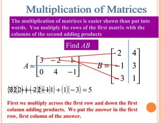
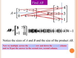


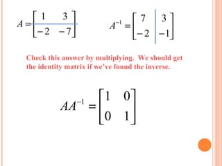
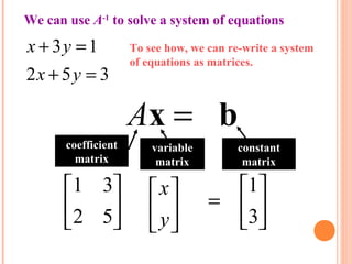


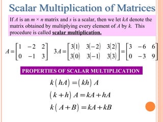
The document discusses matrix algebra and provides examples of key concepts: - A matrix is a rectangular array of numbers or other elements that can be added and multiplied. Matrices are used to represent linear equations and transformations. - The dimensions of matrices must match for multiplication to be defined. Multiplying a matrix by the identity matrix does not change the matrix. - To find the inverse of a matrix A, the matrix is written next to the identity matrix and row operations are performed to reduce A to the identity matrix, yielding the inverse on the right side.


![MATH 564 Advanced Mathematics for Data Science[1].pptx](https://cdn.slidesharecdn.com/ss_thumbnails/math564advancedmathematicsfordatascience1-250915112031-c023a536-thumbnail.jpg?width=640&height=640&fit=bounds)


![Metrix[1]](https://cdn.slidesharecdn.com/ss_thumbnails/metrix1-140722104749-phpapp01-thumbnail.jpg?width=640&height=640&fit=bounds)


