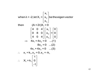
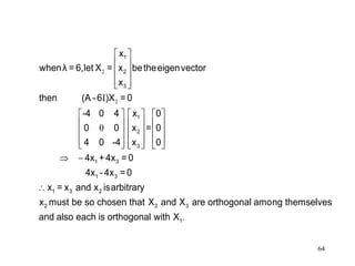
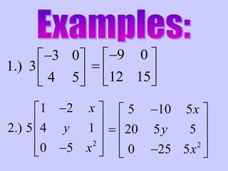
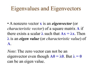
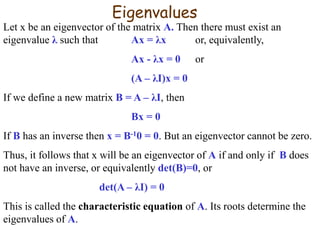
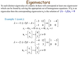
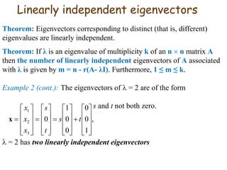
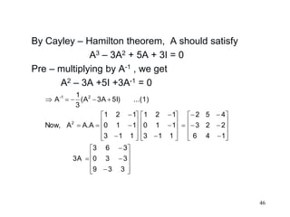
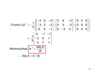
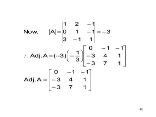
Here are the key steps to find the eigenvalues of the given matrix: 1) Write the characteristic equation: det(A - λI) = 0 2) Expand the determinant: (1-λ)(-2-λ) - 4 = 0 3) Simplify and factor: λ(λ + 1)(λ + 2) = 0 4) Find the roots: λ1 = 0, λ2 = -1, λ3 = -2 Therefore, the eigenvalues of the given matrix are -1 and -2.

2. 11 12 13 14
21 22 23 24
31 32 33 34
1 2 3 4m m m m
a a a a
a a a a
a a a a
a a a a







 
Row 1
Row 2
Row 3
Row m
Column 1 Column 2 Column 3 Column 4

3. A matrix of m rows and n columns is called
a matrix with dimensions m x n.
2 3 4
1.) 1
1
2

  
 
 
 
3 8 9
2.) 2 5
6 7 8

 
  
  
10
3.)
7
 
  
 4.) 3 4
2 X 3
3 X 3
2 X 1
1 X 2

4. 3 5
1
1.) 4
4
0
 
 
 
 
  
3 0
2.)
0 3
 
 
 
1 2 3
3.) 0 1 8
0 0 1
 
 
 
  
4.) 2 
 
5
5.)

 
 
 
 6.) 3
3 X 2 2 X 2 3 X 3
1 X 2 2 X 1 1 X 1

6. To add matrices, we add the corresponding
elements. They must have the same
dimensions.
5 0 6 3
4 1 2 3
A B
    
    
   
A + B
5 6 0 3
4 2 1 3
    
    
1 3
6 4
 
  
 

7. 2 1 3 0 0 0
2.)
1 0 1 0 0 0
   
      
2 1 3
1 0 1
 
  
When a zero matrix is added to another
matrix of the same dimension, that same
matrix is obtained.

8. To subtract matrices, we subtract the
corresponding elements. The matrices must
have the same dimensions.
1 2 1 1
3.) 2 0 1 3
3 1 2 3
   
       
       
1 1 2 ( 1)
2 1 0 3
3 2 1 3
   
    
     
0 3
3 3
5 4
 
    
   

9. 4 1 6 5
1.)
6 3 7 3
     
      
1 3 2 2 1 5
2.)
4 0 5 6 4 3
    
      
2 6
13 0
  
  
 
1 4 7
2 4 8
  
    

10. ADDITIVE INVERSE OF A MATRIX:
1 0 2
3 1 5
A
 
   
1 0 2
3 1 5
A
  
     

11. Find the additive inverse:
2 1 5
6 4 3
 
  
2 1 5
6 4 3
  
    

12. Scalar Multiplication:
1 2 3
1 2 3
4 5 6
k
 
    
  
We multiply each element of the matrix
by scalar k.
1 2 3
1 2 3
4 5 6
k k k
k k k
k k k
 
     
  

13. 3 0
1.) 3
4 5
 
 
 
9 0
12 15
 
  
 
2
1 2
2.) 5 4 1
0 5
x
y
x
 
 
 
  
2
5 10 5
20 5 5
0 25 5
x
y
x
 
   
  

14. • Associative Property of Addition
(A+B)+C = A+(B+C)
• Commutative Property of Addition
A+B = B+A
• Distributive Property of Addition and
Subtraction S(A+B) = SA+SB
S(A-B) = SA-SB
• NOTE: Multiplication is not included!!!

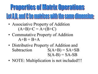
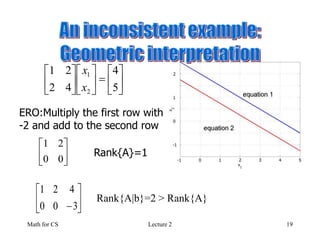
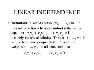
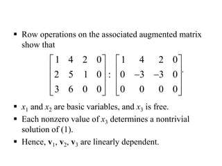
15. • The following operations applied to the augmented
matrix [A|b], yield an equivalent linear system
– Interchanges: The order of two rows/columns can
be changed
– Scaling: Multiplying a row/column by a nonzero
constant
– Sum: The row can be replaced by the sum of that
row and a nonzero multiple of any other row.
One can use ERO and ECO to find the Rank as follows:
EROminimum # of rows with at least one nonzero entry
or
ECOminimum # of columns with at least one nonzero entry

16. Math for CS Lecture 2 16
nnnnnn
nn
nn
bxaxaxa
bxaxaxa
bxaxaxa







2211
22222121
11212111





































nnnnnn
n
n
b
b
b
x
x
x
aaa
aaa
aaa





2
1
2
1
21
22221
11211

(1)

17. bxA 
Each side of the equation
bAxAA 11 

Can be multiplied by A-1 :
Due to the definition of A-1: xxIxAA 1
Therefore the solution of (2) is:
(2)
bAx 1


18. • A-1 does not exist for every A.
• The linear system of equations A·x=b has a
solution, or said to be consistent if
Rank{A}=Rank{A|b}
• A system is inconsistent when
Rank{A}<Rank{A|b}
Rank{A} is the maximum number of linearly independent
columns or rows of A. Rank can be found by using ERO
(Elementary Row Oparations) or ECO (Elementary column
operations).

19. Math for CS Lecture 2 19


















5
4
42
21
2
1
x
x






00
21
Rank{A}=1
Rank{A|b}=2 > Rank{A}
ERO:Multiply the first row with
-2 and add to the second row






3
4
0
2
0
1

20. Math for CS Lecture 2 20
• The system has a unique solution if
Rank{A}=Rank{A|b}= n,
where n is the order of the system.

21. Math for CS Lecture 2 21
• If Rank{A}=n
Det{A}  0  A-1 exists  Unique solution


















 2
4
11
21
2
1
x
x

22. • If Rank{A}=m<n
Det{A} = 0  A is singular so not invertible
infinite number of solutions (n-m free variables)
under-determined system


















8
4
42
21
2
1
x
x
Consistent so solvable
Rank{A}=Rank{A|b}=1

23. • A nonzero vector x is an eigenvector (or
characteristic vector) of a square matrix A if
there exists a scalar λ such that Ax = λx. Then
λ is an eigen value (or characteristic value) of
A.
Note: The zero vector can not be an
eigenvector even though A0 = λ0. But λ = 0
can be an eigen value.
Eigenvalues and Eigenvectors

24. 2 2 4
1 3 6
2 4 2 0
:
3 6 1 0
2 0
0, 0
1 0
, , 0 .
Show x is aneigenvector for A
Solution Ax
But for x
Thus xis aneigenvector of A and is aneigenvalue
 

   
       
     
           
   
     
   

Example:

25. Eigenvalues
Let x be an eigenvector of the matrix A. Then there must exist an
eigenvalue λ such that Ax = λx or, equivalently,
Ax - λx = 0 or
(A – λI)x = 0
If we define a new matrix B = A – λI, then
Bx = 0
If B has an inverse then x = B-10 = 0. But an eigenvector cannot be zero.
Thus, it follows that x will be an eigenvector of A if and only if B does
not have an inverse, or equivalently det(B)=0, or
det(A – λI) = 0
This is called the characteristic equation of A. Its roots determine the
eigenvalues of A.

26. Example 1: Find the eigenvalues of
two eigenvalues: 1,  2
Note: The roots of the characteristic equation can be repeated. That is, λ1 = λ2 =…= λk.
If that happens, the eigenvalue is said to be of multiplicity k.
Example 2: Find the eigenvalues of
λ = 2 is an eigenvector of multiplicity 3.









51
122
A
)2)(1(23
12)5)(2(
51
122
2









 AI
Eigenvalues: examples











200
020
012
A
0)2(
200
020
012
3




 



 AI

27. Example 1 (cont.):





 









00
41
41
123
)1(:1 AI
0,
1
4
,404
2
1
1
2121














tt
x
x
txtxxx
x





 









00
31
31
124
)2(:2 AI
0,
1
3
2
1
2 











 ss
x
x
x
Eigenvectors
To each distinct eigenvalue of a matrix A there will correspond at least one eigenvector
which can be found by solving the appropriate set of homogenous equations. If λi is an
eigenvalue then the corresponding eigenvector xi is the solution of (A – λiI)xi = 0

28. Example 2 (cont.): Find the eigenvectors of
Recall that λ = 2 is an eigenvector of multiplicity 3.
Solve the homogeneous linear system represented by
Let . The eigenvectors of  = 2 are of the form
s and t not both zero.






























 

0
0
0
000
000
010
)2(
3
2
1
x
x
x
AI x
txsx  31 ,
,
1
0
0
0
0
1
0
3
2
1











































 ts
t
s
x
x
x
x
Eigenvectors











200
020
012
A

29. Properties of Eigenvalues and Eigenvectors
Definition: The trace of a matrix A, designated by tr(A), is the sum of the
elements on the main diagonal.
Property 1: The sum of the eigenvalues of a matrix equals the trace of the
matrix.
Property 2: A matrix is singular if and only if it has a zero eigenvalue.
Property 3: The eigenvalues of an upper (or lower) triangular matrix are
the elements on the main diagonal.
Property 4: If λ is an eigenvalue of A and A is invertible, then 1/λ is an
eigenvalue of matrix A-1.

30. Properties of Eigenvalues and
Eigenvectors
Property 5: If λ is an eigenvalue of A then kλ is an eigenvalue of kA
where k is any arbitrary scalar.
Property 6: If λ is an eigenvalue of A then λk is an eigenvalue of Ak for
any positive integer k.
Property 8: If λ is an eigenvalue of A then λ is an eigenvalue of AT.
Property 9: The product of the eigenvalues (counting multiplicity) of a
matrix equals the determinant of the matrix.

31. Linearly independent eigenvectors
Theorem: Eigenvectors corresponding to distinct (that is, different)
eigenvalues are linearly independent.
Theorem: If λ is an eigenvalue of multiplicity k of an n  n matrix A
then the number of linearly independent eigenvectors of A associated
with λ is given by m = n - r(A- λI). Furthermore, 1 ≤ m ≤ k.
Example 2 (cont.): The eigenvectors of  = 2 are of the form
s and t not both zero.
 = 2 has two linearly independent eigenvectors
,
1
0
0
0
0
1
0
3
2
1











































 ts
t
s
x
x
x
x

32. LINEAR INDEPENDENCE
• Definition: A set of vectors {v1, …, vp} in
is said to be linearly independent if the vector
equation
has only the trivial solution. The set {v1, …, vp} is
said to be linearly dependent if there exist
weights c1, …, cp, not all zero, such that
n
1 1 2 2
v v ... v 0p p
x x x   
1 1 2 2
v v ... v 0p p
c c c   

33. • Equation (1) is called a linear dependence
relation among v1, …, vp when the weights are not
all zero. A set is linearly dependent if and only if it
is not linearly independent.
Example 1: Let , , and .
1
1
v 2
3
 
 
 
  
2
4
v 5
6
 
 
 
  
3
2
v 1
0
 
 
 
  

34. a. Determine if the set {v1, v2, v3} is linearly
independent.
b. If possible, find a linear dependence relation
among v1, v2, and v3.
 Solution: We must determine if there is a nontrivial
solution of the following equation.
1 2 3
1 4 2 0
2 5 1 0
3 6 0 0
x x x
       
         
       
              

35.  Row operations on the associated augmented matrix
show that
.
 x1 and x2 are basic variables, and x3 is free.
 Each nonzero value of x3 determines a nontrivial
solution of (1).
 Hence, v1, v2, v3 are linearly dependent.
1 4 2 0 1 4 2 0
2 5 1 0 0 3 3 0
3 6 0 0 0 0 0 0
   
    
   
      
:

36. b. To find a linear dependence relation among v1,
v2, and v3, row reduce the augmented matrix
and write the new system:
• Thus, , , and x3 is free.
• Choose any nonzero value for x3—say, .
• Then and .
1 0 2 0
0 1 1 0
0 0 0 0
 
 
 
  
1 3
2 3
2 0
0
0 0
x x
x x
 
 

1 3
2x x 2 3
x x 
3
5x 
1
10x  2
5x  

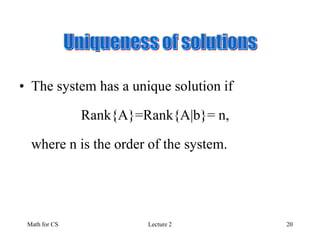
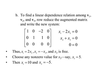
37. CAYLEY HAMILTON THEOREM
Every square matrix satisfies its own
characteristic equation.
Let A = [aij]n×n be a square matrix
then,
nnnn2n1n
n22221
n11211
a...aa
................
a...aa
a...aa
A















38. Let the characteristic polynomial of A be  (λ)
Then,
The characteristic equation is
 
 
 
 
 
 
11 12 1n
21 22 2n
n1 n2 nn
φ(λ) = A - λI
a - λ a ... a
a a - λ ... a
=
... ... ... ...
a a ... a - λ
| A - λI|=0

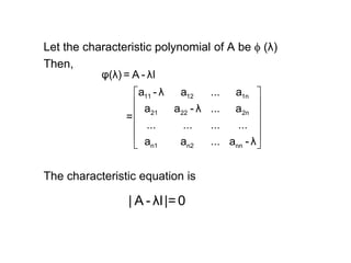
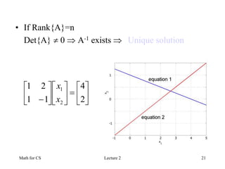
39. Note 1:- Premultiplying equation (1) by A-1 , we
have
 n n-1 n-2
0 1 2 n
n n-1 n-2
0 1 2 n
We are to prove that
p λ +p λ +p λ +...+p = 0
p A +p A +p A +...+p I= 0 ...(1)
I

n-1 n-2 n-3 -1
0 1 2 n-1 n
-1 n-1 n-2 n-3
0 1 2 n-1
n
0 =p A +p A +p A +...+p +p A
1
A =- [p A +p A +p A +...+p I]
p

40. This result gives the inverse of A in terms of
(n-1) powers of A and is considered as a practical
method for the computation of the inverse of the
large matrices.
Note 2:- If m is a positive integer such that m > n
then any positive integral power Am of A is linearly
expressible in terms of those of lower degree.

41. Verify Cayley – Hamilton theorem for the matrix
A = . Hence compute A-1 .
Solution:- The characteristic equation of A is













211
121
112
tion)simplifica(on049λ6λλor
0
λ211
1λ21
11λ2
i.e.,0λIA
23






Example 1:-

42. To verify Cayley – Hamilton theorem, we have to
show that A3 – 6A2 +9A – 4I = 0 … (1)
Now,


















































































222121
212221
212222
211
121
112
655
565
556
655
565
556
211
121
112
211
121
112
23
2
AAA
A

43. A3 -6A2 +9A – 4I = 0
= - 6 + 9
-4
=
This verifies Cayley – Hamilton theorem.














222121
212221
212222













655
565
556













211
121
112










100
010
001
0
000
000
000












44. 44
Now, pre – multiplying both sides of (1) by A-1 , we
have
A2 – 6A +9I – 4 A-1 = 0
=> 4 A-1 = A2 – 6 A +9I



































































311
131
113
4
1
311
131
113
100
010
001
9
211
121
112
6
655
565
556
4
1
1
A
A

45. 45
Given find Adj A by using Cayley –
Hamilton theorem.
Solution:- The characteristic equation of the given
matrix A is














113
110
121
A
tion)simplifica(on035λ3λλor
0
λ113
1λ10
1-2λ1
i.e.,0λIA
23






Example 2:-

46. 46
By Cayley – Hamilton theorem, A should satisfy
A3 – 3A2 + 5A + 3I = 0
Pre – multiplying by A-1 , we get
A2 – 3A +5I +3A-1 = 0
























































339
330
363
3A
146
223
452
113
110
121
113
110
121
A.AANow,
(1)...5I)3A(A
3
1
A
2
21-

47. 47
AAAAdj.
A
AAdj.
Athat,knowWe
173
143
110
3
1
500
050
005
339
330
363
146
223
452
3
1
AFrom(1),
1
1
1





































































48. 48







































173
143
110
AAdj.
173
143
110
3
1
3)(AAdj.
3
113
110
121
ANow,

49. 49
DIAGONALISATION OF A
MATRIX
Diagonalisation of a matrix A is the process of
reduction A to a diagonal form.
If A is related to D by a similarity transformation,
such that D = M-1AM then A is reduced to the
diagonal matrix D through modal matrix M. D is
also called spectral matrix of A.

50. 50
REDUCTION OF A MATRIX TO
DIAGONAL FORM
If a square matrix A of order n has n linearly
independent eigen vectors then a matrix B can
be found such that B-1AB is a diagonal matrix.
Note:- The matrix B which diagonalises A is called
the modal matrix of A and is obtained by
grouping the eigen vectors of A into a square
matrix.

51. 51
Similarity of matrices:-
A square matrix B of order n is said to be a
similar to a square matrix A of order n if
B = M-1AM for some non singular
matrix M.
This transformation of a matrix A by a non –
singular matrix M to B is called a similarity
transformation.
Note:- If the matrix B is similar to matrix A, then B
has the same eigen values as A.

52. 52
Reduce the matrix A = to diagonal form by
similarity transformation. Hence find A3.
Solution:- Characteristic equation is
=> λ = 1, 2, 3
Hence eigen values of A are 1, 2, 3.












300
120
211
0












λ-300
1λ-20
21λ1-
Example:-

53. 53
Corresponding to λ = 1, let X1 = be the eigen
vector then










3
2
1
x
x
x

















































0
0
1
kX
x0x,kx
02x
0xx
02xx
0
0
0
x
x
x
200
110
210
0X)I(A
11
3211
3
32
32
3
2
1
1

54. 54
Corresponding to λ = 2, let X2 = be the eigen
vector then,










3
2
1
x
x
x

















































0
1-
1
kX
x-kx,kx
0x
0x
02xxx
0
0
0
x
x
x
100
100
211-
0X)(A
22
32221
3
3
321
3
2
1
2
0,
I2

55. 55
Corresponding to λ = 3, let X3 = be the eigen
vector then, 









3
2
1
x
x
x

















































2
2-
3
kX
xk-x,kx
0x
02xxx
0
0
0
x
x
x
000
11-0
212-
0X)(A
33
13332
3
321
3
2
1
3
3
2
2
3
,
2
I3
k
x

56. 56
Hence modal matrix is
























 














2
1
00
11-0
2
1-
11
M
MAdj.
M
1-00
220
122-
MAdj.
2M
200
21-0
311
M
1

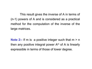
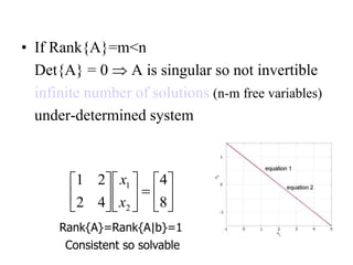
57. 57
Now, since D = M-1AM
=> A = MDM-1
A2 = (MDM-1) (MDM-1)
= MD2M-1 [since M-1M =
I]



















































300
020
001
200
21-0
311
300
120
211
2
1
00
11-0
2
1
11
AMM 1

58. 58
Similarly, A3 = MD3M-1
=
A3 =















































2700
19-80
327-1
2
1
00
11-0
2
1
11
2700
080
001
200
21-0
311

59. 59
ORTHOGONAL TRANSFORMATION
OF A SYMMETRIC MATRIX TO
DIAGONAL FORM
A square matrix A with real elements is said to
be orthogonal if AA’ = I = A’A.
But AA-1 = I = A-1A, it follows that A is orthogonal if
A’ = A-1.
Diagonalisation by orthogonal transformation is
possible only for a real symmetric matrix.

60. 60
If A is a real symmetric matrix then eigen
vectors of A will be not only linearly independent
but also pairwise orthogonal.
If we normalise each eigen vector and use
them to form the normalised modal matrix N then it
can be proved that N is an orthogonal matrix.

61. 61
The similarity transformation M-1AM = D takes
the form N’AN = D since N-1 = N’ by a property of
orthogonal matrix.
Transforming A into D by means of the
transformation N’AN = D is called as orthogonal
reduction or othogonal transformation.
Note:- To normalise eigen vector Xr, divide each
element of Xr, by the square root of the sum of the
squares of all the elements of Xr.

62. 62
Diagonalise the matrix A = by means of an
orthogonal transformation.
Solution:-
Characteristic equation of A is
204
060
402
66,2,λ
0λ)16(6λ)λ)(2λ)(6(2
0
λ204
0λ60
40λ2






Example :-

63. 63
I
 
 
 
  
     
     
     
          


 
   
  
1
1 2
3
1
1
2
3
1 3
2
1 3
1 1 2 3 1
1 1
x
whenλ = -2,let X = x betheeigenvector
x
then (A + 2 )X = 0
4 0 4 x 0
0 8 0 x = 0
4 0 4 x 0
4x + 4x = 0 ...(1)
8x = 0 ...(2)
4x + 4x = 0 ...(3)
x = k ,x = 0,x = -k
1
X = k 0
-1

64. 64
2
2I
0
 
 
 
  
     
     
     
          
 

1
2
3
1
2
3
1 3
1 3
1 3 2
2 2 3
x
whenλ = 6,let X = x betheeigenvector
x
then (A -6 )X = 0
-4 0 4 x 0
0 0 x = 0
4 0 -4 x 0
4x +4x = 0
4x - 4x = 0
x = x and x isarbitrary
x must be so chosen that X and X are orthogonal among th
.1
emselves
and also each is orthogonal with X

65. 65
   
   
   
      


 
 
 
  

2 3
3 1
3 2
3
1 α
Let X = 0 and let X = β
1 γ
Since X is orthogonal to X
α - γ = 0 ...(4)
X is orthogonal to X
α + γ = 0 ...(5)
Solving (4)and(5), we get α = γ = 0 and β is arbitrary.
0
Taking β =1, X = 1
0
1 1 0
Modal matrix is M = 0 0 1
-1 1
 
 
 
  0

66. 66
 
 
 
 
 
 
  
 
  
    
    
    
        
    
 
 
 
  
The normalised modal matrix is
1 1
0
2 2
N = 0 0 1
1 1
- 0
2 2
1 1
0 - 1 1
02 2 2 0 4 2 2
1 1
D =N'AN = 0 0 6 0 0 0 1
2 2
4 0 2 1 1
- 00 1 0
2 2
-2 0 0
D = 0 6 0 which is the required diagonal matrix
0 0 6
.