Downloaded 254 times
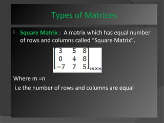
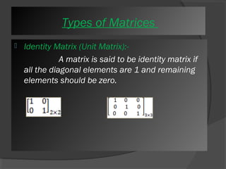
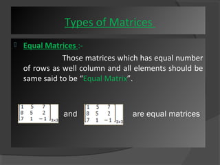
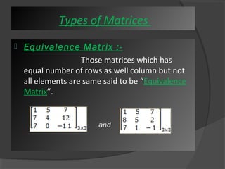
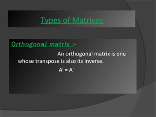
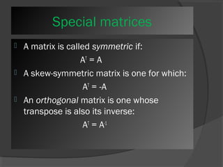
![Types of Matrices
1. Row Matrix : A matrix which has only one row and n
numbers of columns called “Row Matrix”.
Ex : - [ 3 4 6 7 8 ………………n]
2. Column Matrix : A Matrix which has only one column
and n numbers of rows called “column Matrix”.
3567....n](https://image.slidesharecdn.com/matrixalgebra1-141028075845-conversion-gate02/85/Matrix-and-its-applications-by-mohammad-imran-21-320.jpg)

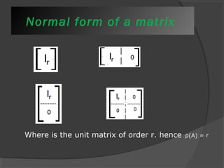

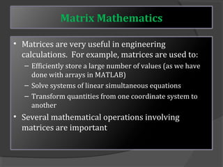
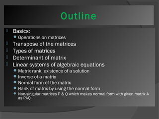
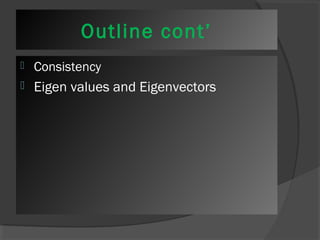
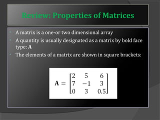
This document provides an overview of matrix mathematics concepts. It discusses how matrices are useful in engineering calculations for storing values, solving systems of equations, and coordinate transformations. The outline then reviews properties of matrices and covers various matrix operations like addition, multiplication, and transposition. It also defines different types of matrices and discusses determining the rank, inverse, eigenvalues and eigenvectors of matrices. Key matrix algebra topics like solving systems of equations and putting matrices in normal form are summarized.