This document introduces some useful functions in Microsoft Excel 2003. It discusses counting functions like COUNT, COUNTA, COUNTBLANK and COUNTIF that count the number of cells meeting certain criteria. Logical functions like IF, AND, OR and NOT are also covered. IF allows alternative results depending on a condition, AND checks if multiple criteria are true, OR checks if any criteria are true, and NOT changes true to false and vice versa. COUNTIF works similarly to IF but counts cells meeting the criteria. SUMIF adds up cells that meet provided criteria. Examples are provided to demonstrate how to use these functions to analyze data in a spreadsheet.

1. Some Useful Functions in Microsoft Excel 2003
Introduction
Most users should be familiar with functions as they first encountered them at
school in mathematics lessons - for example when working out square roots,
SQRT(...), or logarithms, LOG(...). They are often used to perform quite
complex calculations, without the user having to know how this is done. At
school, the answers often had to be looked up manually in a book of tables; in
Excel, the calculations are done automatically for you.
Functions have a set structure, starting with the function name then,
surrounded by round brackets, what is known as the argument. Functions in
Excel follow exactly the same pattern, though they often have more than one
argument, each of which is separated by a comma.
In all, Microsoft Excel provides over 300 different functions covering a wide
range of needs. Many are geared up to industry and commerce (including
some very specialist financial ones) but there are also many of use to the
average Excel user. Some functions were introduced on the Beginners' course,
eg SUM(...) and IF(...), while AVERAGE(...) was used in the Intermediate
training.
This document looks at some of the more commonly-used functions and
shows you how they work. It also shows you how to define and create your
own custom-built functions.
Entering a Function
Functions are entered into a formula in a cell in much the same way as a cell
reference or data value. All formulae must be started with an equals sign,
followed by the calculation. This may just be a function or a function embedded
in other data values and/or cell references. Functions can be typed in directly
or use can be made of the Insert Function toolbar button. The most
commonly-used function is SUM(...), which has its own (AutoSum) button.
Other functions can be accessed using the list arrow attached to this button.
1. Start up Excel as usual and [Open] the file advanced.xls in the
D:Training folder
2. Move to the Accounts sheet by clicking on its tab

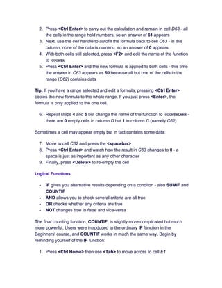
2. 3. Press <Ctrl End> to move to the end of the data then <down arrow> to
move to cell D62
4. Click on the [AutoSum] toolbar button then press <Ctrl Enter> (this key
combination enters the formula AND stays in the same cell)
5. Repeat step 4 but this time use the list arrow attached to [AutoSum] and
choose Max or Min or Average - try them all, if you like
6. <Delete> the result and then try using the [Insert Function] button
(shown as [fx]) on the Formula Bar instead - the Insert Function window
appears:
Note: You can also get this window by choosing More Functions from the
[AutoSum] list.
7. Click on [OK] to insert the SUM function - the Formula Palette appears

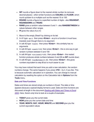
3. The Formula Palette
The Formula Palette can be a great aid, especially for functions you are less
familiar with. It provides guidance on the use of each function and its
arguments. The arguments appear at the top of the window with information on
each appearing below as you fill in the boxes - SUM, for example, can only be
used to add up 30 number ranges or separate cells and text is ignored. Should
you need further help (and examples of its use), a Help on this function link is
provided in the bottom left corner of the window.
At the foot of the palette, the Formula result appears. If this doesn't give you
what you want then you know you are trying to use the function incorrectly and
an error message may be shown against one of the arguments.
1. Type d1:d61 to change the Number1 argument - note that the column
heading Amount is now included but the Formula result hasn't changed
2. Press <Enter> for [OK] to insert the function
3. Press <F2> to enter edit mode and amend the formula to read
=SUM(d1:d6,d40,d50:d61) - note how each separate cell range or cell is
colour coded so that you can check you have the right ones
4. Press <Ctrl Enter> to carry out the calculation then click on the [Insert
Function] button to display the Formula Palette and see how the list of
arguments has changed
5. Press <Enter> for [OK] to re-enter the formula
Note how you can specify non-adjacent single cells and cell ranges in a
function by separating them by commas.

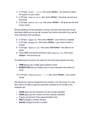
4. Frequently-Used Functions
The following exercises introduce you to many of the most useful and
commonly-used functions. It obviously isn't possible to explore everything; just
be aware as to what's available. The Insert Function window lets you Search
for a function. It also divides functions up into various categories: financial,
date & time, math & trig, statistical, lookup & reference, database, engineering,
logical, information and text. You can also create your own User Defined
functions, as you'll see later.
To see a list of all the functions:
1. Press <down arrow> to move to cell D63
2. Click on the [Insert Function] button then on the list arrow attached to Or
select a category:
3. Note the categories available (you'll be covering some of these in a minute)
then select All
4. Hold down the mouse button on the arrow at the foot of the Select a
function: scroll bar to move down the list
5. If you'd like to know more about any function, select it from the list and
read the brief description provided - use the Help on this function link to
get full details
6. End by closing down the Insert Window button - click on [Cancel] or press
<Esc>
Now let's look at some of the more useful functions in detail.
Counting Functions
There are four functions which let you count up the number of cells matching
certain criteria:
• COUNT tells you how many cells contain numbers
• COUNTA tells you how many cells are not empty
• COUNTBLANK tells you how many cells are empty
• COUNTIF tells you how many cells match a certain criterion
There are also two specialised functions (DCOUNT and DCOUNTA) for when
Excel is used as a database.
1. Click on the list arrow attached to [AutoSum] and choose Count

5. 2. Press <Ctrl Enter> to carry out the calculation and remain in cell D63 - all
the cells in the range hold numbers, so an answer of 61 appears
3. Next, use the cell handle to autofill the formula back to cell C63 - in this
column, none of the data is numeric, so an answer of 0 appears
4. With both cells still selected, press <F2> and edit the name of the function
to COUNTA
5. Press <Ctrl Enter> and the new formula is applied to both cells - this time
the answer in C63 appears as 60 because all but one of the cells in the
range (C62) contains data
Tip: If you have a range selected and edit a formula, pressing <Ctrl Enter>
copies the new formula to the whole range. If you just press <Enter>, the
formula is only applied to the one cell.
6. Repeat steps 4 and 5 but change the name of the function to COUNTBLANK -
there are 0 empty cells in column D but 1 in column C (namely C62)
Sometimes a cell may appear empty but in fact contains some data:
7. Move to cell C62 and press the <spacebar>
8. Press <Ctrl Enter> and watch how the result in C63 changes to 0 - a
space is just as important as any other character
9. Finally, press <Delete> to re-empty the cell
Logical Functions
• IF gives you alternative results depending on a conditon - also SUMIF and
COUNTIF
• AND allows you to check several criteria are all true
• OR checks whether any criteria are true
• NOT changes true to false and vice-versa
The final counting function, COUNTIF, is slightly more complicated but much
more powerful. Users were introduced to the ordinary IF function in the
Beginners' course, and COUNTIF works in much the same way. Begin by
reminding yourself of the IF function:
1. Press <Ctrl Home> then use <Tab> to move across to cell E1

6. 2. Type '+VAT (don't forget the single quote or you will get an error message)
then press <down_arrow>
3. In cell E2 type =if( then click on the [Insert Function] button
Tip: If you type in the name of a function and its opening bracket, you can use
this method to display the function palette to help you with the arguments.
4. Set the Logical_test to c2="food" - note the argument is FALSE as C2
holds the text Stationery
5. Set the Value_if_true to d2 and the Value_if_false to d2*115%
6. Press <Enter> for [OK] - VAT at 15% is added to the cost
7. Double click on the cell handle to autofill the formula in cell E2 down the
column
8. You don't want to include cells E62 and E63, so use the cell handle to
shrink the copied area so that it ends at cell E61
Except where Food is the Category, you now have VAT at 15% added to the
Amount.
9. Finally, select column D by clicking on the column heading then click on
the [Format Painter] button
10.Copy the format of the cells in column D to the next column by clicking on
the E column heading
Next, investigate COUNTIF:
1. Move to cell C63 and replace the current contents by typing Food
2. Move to D63 (<right arrow>) and type =countif( then click on [Insert
Function] for assistance
3. Set the Range to c2:c61 and Criteria to "food" - when counting words
you must enclose the text in quotation marks
4. Press <Enter> for [OK] - 22 of the cells in the range contain the word
Food
There's an equivalent function for adding up cells matching certain criteria,
namely, SUMIF:
5. Move to E63 (<right arrow>) and type =sumif( then click on [Insert
Function] for assistance

7. 6. Set the Range: to c2:c61,as before, and Criteria to c63
7. Finally set the Sum_range to d2:d61 then press <Enter> to complete the
formula
You now know that the total spent on food was £149.08. In fact there are
easier ways to get this information, as you'll see later.
8. End by changing C63 to travel - you now have the total spent on travel
There are 3 more logical functions to consider, namely AND, OR and NOT:
1. Press <Ctrl Home> to move to the top of the sheet then click on cell F2
2. Type =AND( then click on the [Insert Function] button
3. Set Logical1 to b2="Liz" and Logical2 to c2="Food"
Although the first criteria is TRUE, the second isn't, so the result of the formula
is also FALSE.
4. Press <Enter> to complete the formula then double click on the cell
handle to autofill down the column - only a couple of cells in column F give
the result as TRUE
5. With the cells still selected, press <F2> and edit the formula to read OR
instead of AND
6. Press <Ctrl Enter> to copy the new formula down the column - this time a
result of TRUE is shown if either the value in column B is Liz or that in
column C is Food
Nested Functions
One function can be used inside another. This is called nesting. For example,
you can reverse the results in column F by nesting the OR function inside a
NOT function:
1. With the cells still selected, press <F2> and edit the formula to read
=NOT(OR(B2="Liz", C2="Food")) - don't forget the final extra bracket
2. Press <Ctrl Enter> to copy the new formula down the selection
You can't always nest one function inside another - for example, you can't use
the logical functions in SUMIF() or COUNTIF().

8. 3. Press <Ctrl down arrow> to move to the bottom of column F then <down
arrow> again to make F62 the active cell
4. Type =countif(c2:c61,NOT("food")) then press <Ctrl Enter> - the
formula result is 0, which is obviously wrong
5. Click on the [Insert Function] button and note the red #VALUE! error
message against Criteria
Here, you can't use the NOT() function, but you could use the not equal (<>)
mathematical operator - though even this isn't straightforward:
6. Edit the Criteria to read "<>Food" - because you are counting text, the
criteria must also be text
7. Press <Enter> for [OK] - the formula result is now correct, namely 38
Functions which convert numbers to text (and vice-versa) are dealt with later in
this document.
In cases where nesting is not allowed (or becomes too complex so that it's
difficult to understand what's going on), you may need to carry out the
calculations in two stages. Here, for example, you already have a column
using the logical functions, which you can use to carry out your calculations:
8. Click on the [Insert Function] button then reset the Range to f2:f61 and
Criteria to true
9. Press <Enter> for [OK] to count the number of rows without either Liz in
column B or Food in column C
Filtering and the SUBTOTAL Function
Being able to get answers depending on a condition (as with SUMIF) is really
useful but, as you've seen, it's not easy to set up multiple conditions. It's much
easier to use filters and the SUBTOTAL function:
1. Begin by deleting rows 62 and 63 - drag through the row numbers to
select them, then open the Edit menu and choose Delete
2. Press <Ctrl Home> then open the Data menu, choose Filter then
AutoFilter
3. Press <down arrow> to move to cell A2, open the Window menu and
choose Freeze Panes
4. Click on the list arrow in C1 and choose Stationery

9. 5. Move to D62 then click on the [AutoSum] button - the function
SUBTOTAL(9,D2:D61) appears
6. Press <Ctrl Enter> and the total of the filtered values is worked out
7. Click on the list arrow in B1 and choose Emma - you now know what
Emma spent on stationery
8. Change the criteria by selecting different values in B1 and C1
The SUBTOTAL function can also give you other measurements (eg
AVERAGE):
9. With D62 the active cell, click on [Insert Function] then on Help on this
function
You'll discover that if the Function_num is 1 (or 101) then you get AVERAGE.
A value of 2 (or 102) is COUNT, 3 is COUNTA, 4 is MAX and 5 is MIN. The
remaining setting values are for more complicated statistical functions.
10.Change the Function_num from 9 to 2 then press <Enter> for [OK] - you
have counted the occurrences
11.Try finding the largest (MAX) and smallest (MIN) values by repeating
steps 9 and 10
12.End by turning off the filtering - open the Data menu, choose Filter then
AutoFilter
13.Finally, close down the on-line Help by clicking on its Close button
Note: A much better way to get summaries of the data like this is to use a
Pivot Table (see Using Pivot Tables in Excel 2003). For more information on
using filters see Using Filters in Excel 2003.
Mathematical Functions
All the functions you met in maths lessons at school are provided in Excel - eg
SQRT(), LOG(), EXP(), SIN() etc - plus many more. The ones discussed below
are useful not just in mathematics.
• ABS makes a number positive if it is negative

10. • INT rounds a figure down to the nearest whole number (ie removes
decimal places) - other similar functions are CEILING and FLOOR, which
round up/down to a multiple such as the nearest 10 or 100
• ROUND rounds a figure to a specified number of digits - also ROUNDUP,
ROUNDDOWN and TRUNC
• RAND gives a random value between 0 and 1 - also RANDBETWEEN for
values between other ranges
• PI gives the value of pi (π)
1. Move to the empty Sheet1 by clicking on its tab
2. In A1 type =pi() then press <Enter> - as pi is a function it must have
brackets even though there is no argument
3. In cell A2 type =rand() then press <Enter> - this similarly has no
arguments
4. In cell A3 type =rand()*100 then press <Enter> - this is one way to get
random numbers between 0 and 100
5. In cell A4 type =int(rand()*100) then press <Enter> - this nested
function produces whole numbers between 0 and 99 as INT rounds down
6. In cell A5 type =randbetween(0,99) then press <Enter> - this gives
numbers equivalent to step 5 but is much easier to use
You may have noticed that each time you add a new calculation, the random
numbers change. The same happens if you press <F9> - try it, if you like. This
is because automatic calculation is in operation. You can change to manual
calculation by resetting the option on the Calculation tab in Options from the
Tools menu.
Date and Time Functions
Dates and times are stored simply as numbers in Excel. The date or time
appears because a special display format is used. Date and time functions are
discussed at length in the document Dealing with Dates and Times in Excel
2003. Here, there's only time to look at a couple of examples:
• TODAY gives you the current date
• NOW gives you the current date and time
• YEAR, MONTH, DAY, HOUR, MINUTE and SECOND give you the
current equivalent values

11. • DAYS360 gives you the number of days between two dates - also
NETWORKDAYS gives the number of working days (excluding weekends)
1. Move to B1 and type =today() then press <Enter> - today's date appears
2. In B2 type =now() then press <Enter> - you get both the date and time
3. To get just the time, in B3 type =now() and press <Ctrl Enter> then open
the Format menu and choose Cells...
4. On the Number tab, choose the Category: Time and select the format
required from Type: then press <Enter> for [OK] - note that there is a
TIME function but it doesn't work as you might expect
5. Move to B4 and type =year(now()) then press <Enter> - you get the
current year (try the other related functions, eg DAY, if you like)
6. To find out how long you've lived, in B5 type
=days360("your_date_of_birth",now()) then press <Enter> - note that
your date of birth must be in quotes and in a recognised date format (eg
25/12/1980 or 25 Dec 1980)
Tip: The easiest way to enter today's date into a cell is to press <Ctrl ;>.
Similarly, <Ctrl :> gives you the current time. Note, however, that the values
are fixed and are not recalculated next time you open the file.
Text Functions
There are also several useful functions for use with text:
• LEN counts the number of characters (including spaces) in the text
• FIND gives the position of the specified text in the text being searched
• LEFT, MID, RIGHT let you select part of the text from the left, middle or
right
• LOWER, UPPER, PROPER change case (lowercase, uppercase, mixed
case)
• EXACT compares the contents of two cells to see if they are exactly the
same
1. First, you need some text to work on, so in C1 type your name then press
<Enter>
2. In C2 type =len(c1) then press <Enter> - this counts the letters (+
spaces) in your name

12. 3. In C3 type =find(" ",c1,1) then press <Enter> - this works out where
the space is in your name
4. In C4 type =left(c1,c3-1) then press <Enter> - this gives you just your
first name
5. In C5 type =mid(c1,c3+1,c2) then press <Enter> - this gives you the rest
of your name
Strictly speaking, the last example is wrong in that the third argument should
have been c2-c3 and not just c2, however the function still works if you ask for
more characters than necessary.
6. In C6 type =upper(c1) then press <Enter> - your name is in capitals
7. In C7 type =proper(c6) then press <Enter> - your name is back to
normal
8. In C8 type =exact(c7,c6) then press <Ctrl Enter> - the cells do not
match
9. Press <F2> and edit the formula to read =exact(c7,c1) then press
<Enter> - this time they do
The following two functions are useful for removing extra spaces from text:
• TRIM leaves just a single space between words
• SUBSTITUTE lets you replace one or more characters with others (or
none)
10.In C9 type =substitute(c6," ","") then press <Enter> - your names
merge
Sometimes you need to change text into numbers, and vice-versa. You may
also need to be able to specify a particular character by its number in the
character set:
• CHAR gives you the character from the number specified
• CODE gives you the number from the character specified
• T gives you text only if the argument itself is textT
• TEXT changes a number into text
• VALUE changes text into a number

13. 11.In C10 type =code("a") then press <Enter> - the letter a is number 97 in
the character set
12.In C11 type =char(98) then press <Enter> - guess what's the letter
following a!
13.In C12 type =32.5&char(176) then press <Enter> - a degree sign is
added to the figure
14.In C13 type =T(c12) then press <Enter> - you still get 32.5°, which
shows the figure in C12 has been stored not as a number but as text (this
should already have been apparent as the value appeared on the left of
the cell)
15.In C14 click on the [AutoSum] button and press <Enter> - the answer
doesn't include the values in C12 or C13
16.Move up to C10 and press <F2> then edit the formula to read
=TEXT(CODE("a"),"#") and press <Enter> - the sum is now 0 as the
number in C10 has been converted to text
17.Move down to C11 and type =VALUE(c10) and press <Enter> - the sum is
again 97 because C11 has converted the text in C10 to a number
The TEXT function needs a little further investigation as it can be a very
powerful function if you know how it works:
18.Move left to cell B10 and type =TEXT( then click on the [Insert Function]
button
19.For the Value type now() then press <Tab> to move to Format_text
The Format_text argument is a set of characters which determines the output
display for the number generated by the TEXT function. This could be a
number, time or date. The characters used match those used in the Format
Cells window (which you'll look at in a minute). The # sign used above
represents any number, without specifying a format. A 0 is used where a
number must be shown - eg #.00 will display the number to 2 decimal places
(even when it's a whole number). In dates, d is used for days, m for months
and y for years. For times, h, m and s are used - see Dealing with Dates and
Times in Excel 2003 for full details.
20.For the Format_text type "dddd" then press <Ctrl Enter> - the result
should tell you what day of the week it is

14. 21.Press <F2> and replace NOW() with your date of birth (in quotes, as
before) to discover what day of the week you were born on - press <Ctrl
Enter>
22.Finally, open the Format menu and choose Cells... then at the bottom of
the Category: list choose Custom
23.Use the scroll bar to see what format codes are available then click on
[Cancel]
If you want to know exactly how everything works, look up custom format in the
Help system.
Lookup & Reference Functions
The final group of Excel functions dealt with in this document are called
Lookup & Reference. These let you search for a value in a specified range - for
example, if you know someone's name you could use a function to give you
their date of birth from a neighbouring column. These functions aren't always
that easy to use and it helps to make use of the Formula Palette.
• MATCH finds the row or column in which a value is stored in a one
dimensional array
• INDEX returns the value specified by the row plus column reference
• HLOOKUP and VLOOKUP combine the above but in a fairly complicated
way
1. In cell A12 type Brass then press <Enter>
2. In A13 type =match( then click on the [Insert Function] button
3. Set the Lookup_value to a12 - press <Tab>
4. For the Lookup_array, click on the students tab (to move to that worksheet)
then on the letter B at the top of the second column - press <Tab>
5. Set the Match_type to 0 and press <Enter> - 0 gives you an exact match
The result (44) tells you that the word Brass was found in row 44 of the column.
6. Move to cell A14 and type =INDEX(data,a13,10) and press <Ctrl Enter>
7. The number needs to be converted to a date so open the Format menu,
choose Cells... then under Category: select Date - you can also change
the Type: if you want

15. 8. Press <Enter> for [OK] and you have the date of birth of Mr Brass
The example needs a little further explanation. The word data in the INDEX
function refers to a named data range. This has already been set up for you
and refers to all the information on the students' sheet. Dates of birth are
stored in column J - the 10th one in the data area.
9. Move to cell A12 and type Cox then press <Enter> - you now have Miss
Cox's date of birth
HLOOKUP and VLOOKUP work on a two-dimensional data area, returning the
value in a specified column or row which corresponds to certain value in
another row or column. Essentially they combine MATCH and INDEX. There
are restrictions in how they work, however:
• The lookup data must be in the left column (or top row) of the array
• The data must also be sorted alphabetically, A to Z
To see how a lookup function works, try repeating the above exercise:
10.Move to cell B14 and type =vlookup( then click on the [Insert Function]
button
11.For the Lookup_value type a12 then press <Tab>
12.For the Table_array, click on the students tab then type b:j (ie
students!b:j) - you need to exclude column A as VLOOKUP works on
the left column
13.Press <Tab>, then for the Col_index_num, type 9 and press <Enter> for
[OK]
14.Finally, move to A14, click on the [Format Painter] then click on B14 to
turn the number into a date - it should match the value in A14
The function worked because both of the conditions mentioned above were
met. To see what happens if this is not the case, try looking up the date of birth
given a student's userid:
15.In A14, edit the formula to read =INDEX(data,A13,7) - press <Enter>
16.Using the cell handle, copy the formula in B14 down to B15 then edit B15
to read =VLOOKUP(A14,students!G:J,4) - press <Enter>

16. Even though you have adjusted the formula to make column G the leftmost in
the Table_array, you'll find you have a different date of birth (11/03/1978
instead of 22/01/1975). The reason for this is that the userid information is not
sorted.
17.Click on the students tab, to move to the data, then click on any cell in
column G
18.Now click on the [Sort Ascending] button to sort by userid
19.Finally, click on the Sheet1 tab and examine the results
You'll find the date of birth is now correct (22/01/1975) in cell B15 but has gone
wrong in cell B14 (because the VLOOKUP function here relies on the data
being sorted by column B).
Hopefully, this example has demonstrated how great care must be taken when
using LOOKUP functions. They are fine where data is fixed (and, better still,
protected) but dangerous where the data might be sorted on a different column
or row.
User-Defined Functions
You can create your own functions in Microsoft Excel. Doing so involves
writing a little program in the Visual Basic Editor. At first sight, this looks very
complicated but you can also use it simply, without knowing anything about
computer programming. This next example creates a function to generate
random numbers which don't change:
1. Open the Tools menu and choose Macro then Visual Basic Editor (don't
be alarmed by the complexity of the window that appears)
2. Now open the Insert menu and choose Module
3. Define the function (its name and arguments) by typing function myrnd(x)
then press <Enter> - the Editor will automatically add a line reading End
Function
4. Now type in the required calculation, using the function name on the left-
hand side to store the result - type: myrnd = rnd() * x
5. Close the Editor by clicking on the red [Close] button - your function is
automatically saved

17. 6. Finally, in cell B16 type =myrnd(100) and press <Enter> - you should get
a random number between 0 and 99.99
7. Press <F9> - note how the number doesn't change, in contrast to those in
A2 to A5
The reason the number doesn't change is because you are using the Visual
Basic function RND() not the Excel function RAND(). This particular function
always gives you the same sequence of numbers (which can be useful - it's
their distribution which is random). You can get genuinely random numbers by
adding some extra code.
To edit one of your own functions:
1. Open the Tools menu and choose Macro then Visual Basic Editor
2. Add a new second line which just says randomize
3. Next, edit the original function calculation to read myrnd =
int(rnd()*x)/10
4. Close the Editor by clicking on the red [Close] button
5. Move up to cell B16 and press <F2> then <Enter> - you should get a
random number with one decimal place between 0.0 and 9.9 (only by re-
entering the formula does the value change)
If you want to use an Excel function in Visual Basic then you have to declare it
as such. This final example works out the area of a circle using the PI()
function:
1. Open the Tools menu and choose Macro then Visual Basic Editor
2. Click below the existing funtion and type function myarea(r) then press
<Enter>
3. Now type in the calculation: myarea = worksheetfunction.pi * r *r
You'll find that as soon as you press the period (full stop) after workfunction
that a list of the available functions appears. You can select from the list or
continue typing.
4. Close the Editor by clicking on the red [Close] button
5. In cell B17 type =myarea(10) then press <Enter> - you have the area of a
circle, radius 10

18. You can have as many functions as you like. By default, they are only stored
within a particular file but Excel does let you save them to be accessible to any
Excel file. Sadly, this feature isn't available on the University lab PCs.