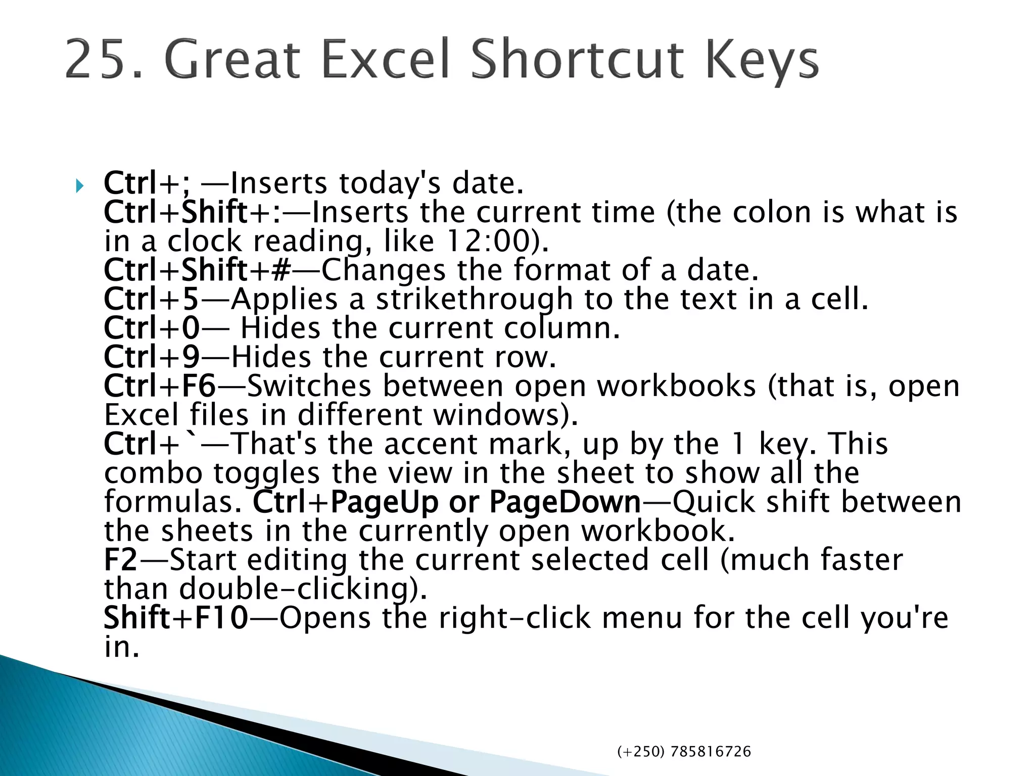
Presentation by:
Mzee. Theogene KUBAHONIYESU
Email: theogenek9@gmail.com
+250785816726
Learn as you Grow up
 Almost all the work that people do in offices is
done with the help of a magical program called
Microsoft Excel, when you first look at it it might
look like a program with only tables and slots for
entering data, but this description does not
suffice for the real capability of this program.
Excel can do anything from managing your office
accounts to managing the data required for
managing a whole country, you just need to
know how to use it. Here in this article a few
really cool Excel tips and tricks are mentioned
that can help many users to improve the way in
which they have used excel till date.
(+250) 785816726
 We can add diagonal lines in our cells by a
simple method of formatting that excel
allows. For this all we need to do is select a
cell in which we wish to add a diagonal line,
upon selecting the cell we would need to
open the options by right clicking on the
mouse. In the options we would need to click
on the option of Format Cells.
(+250) 785816726
(+250) 785816726
 When we click on the Format cells option,
we’ll see a dialog box, in which we’ll need to
click on the border option, highlighted by
red, in the top strip. Then we can click on the
other highlighted option that shows us the
format of a diagonal line in the cell, there is
another one in the dialog box that you can
find on your own.
(+250) 785816726
 Whenever we use excel to enter data into our tables in the
form of numbers, we see certain statistics or a kind of
summary in the status bar below, usually it will carry
the average, count and sum of the data that we select at any
given point of time.
 Excel gives us certain more options for the summary that we
get in the status bar, to exploit it to the maximum, one can do
this by right clicking anywhere on the status bar, once you
right click on the status bar, you’ll see a lot of options among
which would be the additional options that excel provides us
for the summary of data that we have selected. We can choose
from Average, Count, Numerical Count, Minimum, Maximum
and Sum. In the image we can see how our status bar looks
when we select to view most of the options available to us.
(+250) 785816726
 There is a small function that we can use to
transform the case of our text, the function is
quite easy to use, all you need to do for this
is that you need to type ‘UPPER(text/cell)’ for
upper case, ‘Lower(text/cell)’ for lower case
and finally ‘Proper(text/cell)’ for making the
first letter of the word capital. Its usage can
be seen in the images below, with cells
showing Upper, Lower and proper usage
along with the final output that they achieve
from it.
(+250) 785816726
 We can add text from different cells to a
single cell by simply using ’&’, for this all we
need to do is start writing in the cell with ‘=’
and then click on the cells one by one that we
need to add to our new cell, we would also
need to add’&’ after we click on each cell to
be added, as it will add the name of the cell
that we have clicked. So it will look something
like the one in the image below.
(+250) 785816726
 If you suffer from a habit of using SMS or in other
words short hand language everywhere you type, or if
you have a bad history of making spelling errors for
some particular words, then you can use the auto-
correct feature of MS Excel at your convenience. For
using it you’ll first need to go
to File>Options>Proofing>AutoCorrect Options. Here
you’ll see a dialog box that will allow you to enter a
text to be replaced with the text you would want to
replace it with. You can add any words that you
misspell, for example I can put ‘frnz’ as a word to be
replaced by the word ‘friends’, and every time I use
the wrong spelling(frnz), autocorrect will correct
me(by putting friends in its place).
(+250) 785816726
 Conditional formatting is a powerful tool that
excel incorporates, as the name suggests,
conditional formatting formats cells on
certain conditions, for instance, if we had to
highlight the students who have failed in an
exam in the class with red, then we would use
conditional formatting.
(+250) 785816726
 We know how to get a transposed copy of our
data, if some of you don’t then don’t worry all
you need to copy the data you want to transpose
and then while pasting look for paste options
and then click on transpose, you’ll get a
transposed version. This being a kind of normal
copy and paste operation will only create a fixed
transposed version of the original table. so the
equation to be entered becomes
‘=Transpose(A1:B9)’, upon entering this equation
you’ll need to press ‘Shift+Ctrl+Enter’, and you’ll
see the magic happen.
(+250) 785816726
 Sparkline microcharts are small graphs or
charts that you can place in a cell. They were
introduced in MS Word 2010 and can greatly
enhance the view-ability of our excel data. To
make one, you need to first select the data
from which you wish to create a sparkline,
and then go to Inset>Line.
(+250) 785816726
 The count formula counts the number of cells
in a range that have numbers in them.(This
formula only works with numbers though
 Counts the number of non-empty cells in a
range. It will count cells that have numbers
and/or any other characters in them.
 The COUNTA Formula works with all data
types. It counts the number of non-empty
cells no matter the data type.
(+250) 785816726
 The LEN formula counts the number of
characters in a cell. Be careful though! This
includes spaces.
(+250) 785816726
 Formulas: = RIGHT(text, number of characters),
=LEFT(text, number of characters), =MID(text, start
number, number of characters).
 (Note: In all of these formulas, wherever it says “text”
you can use a cell reference as well)
 These formulas return the specified number of
characters from a text string. RIGHT gives you
the number of characters from the right of the text
string, LEFT gives you the number of characters from
the left, and MID gives you the specified number of
characters from the middle of the word. You tell the
MID formula where to start with the start_number and
then it grabs the specified number of characters to
the right of the start_number.
(+250) 785816726
 Formula: =IF(logical_statement, return this if
logical statement is true, return this if logical
statement is false)
 When you’re doing an analysis of a lot of data
in Excel there are a lot of scenarios you could
be trying to discover and the data has to
react differently based on a different
situation.
(+250) 785816726
 Formulas: =SUMIF(range, criteria, sum_range),
=COUNTIF(range, criteria), =AVERAGEIF(range,
criteria, average_range)
 These formulas all do their respective functions
(SUM, COUNT, AVERAGE) IF the criteria are met.
There are also the formulas: SUMIFS, COUNTIFS,
AVERAGEIFS where they will do their respective
functions based on multiple criteria you give the
formula.
 I use these formulas in our example to see the
average revenue (AVERAGEIF) if a person met
their quota, Total revenue (SUMIF) for the just the
sales people who met their quota, and the count
of sales people who met their quota (COUNTIF)
(+250) 785816726
 A fancy word for combining data in 2 (or more)
different cells into one cell. This can be done
with the Concatenate excel formula or it can be
done by simply putting the & symbol in between
the two cells. If I have “Steve” in cell A1 and
“Quatrani” in cell B1 I could put this formula:
=A1&” “&B1 and it would give me “Steve
Quatrani”. (The “ “ puts a space in between
what you are combining with the &). I can use
=concatenate(A1, “ “, B1) and it will give me the
same thing: “Steve Quatrani”
(+250) 785816726
Open a spreadsheet Ctrl+O
Go to the Home tab Alt+H
Save a spreadsheet Ctrl+S
Copy Ctrl+C
Paste Ctrl+V
Undo Ctrl+Z
Remove cell contents Delete key
Choose a fill color Alt+H, H
Cut Ctrl+X
Go to Insert tab Alt+N
Bold Ctrl+B
(+250) 785816726
Bold Ctrl+B
Center align cell contents Alt+H, A, then C
Go to Page Layout tab Alt+P
Go to Data tab Alt+A
Go to View tab Alt+W
Open context menu Shift+F10,
Add borders Alt+H, B
Delete column Alt+H,D, then C
Go to Formula tab Alt+M
Hide the selected rows Ctrl+9
Hide the selected columns Ctrl+0
(+250) 785816726
 =index(d5:h8,match(g14,c5:c8,0),match(h14,
d4:h4,0))
 Return the value or reference of the cell at the
intersection of a particular and column in a
given range.
(+250) 785816726
 Return the value if-error is an error and the
value of the expression itself otherwise.
Returns a value you specify if a formula
evaluates to an error; otherwise, returns the
result of the formula. Use the IFERROR
function to trap and handle errors in a
formula.
(+250) 785816726
 Printing Excel paper has been considered as a
Difficulty work but it is obviously clear and
easy.
Print an Excel table
 Click a cell within the table to activate the
table.
 Click File, and then click Print. Keyboard
shortcut You can also press CTRL+P.
 Under Settings, click Selected Table.

(+250) 785816726
Create a drop down list of items in a cell, with
Excel's Data Validation feature. This will make
data entry easier, and reduce input errors and
typing mistakes.
(+250) 785816726
 Let us construct a Database that should help
a company ,organization or any Business
easily calculates it’s Expenses, Incomes
,debts and Credits.
 Did you know that you can financially control
the Business using one Excel file with
multiple sheets linked together.
(+250) 785816726
 You may want to see certain rows or columns all
the time in your worksheet, especially header
cells. By freezingrows or columns in place, you'll
be able to scroll through your content while
continuing to view the frozen cells.
 Select the row below the row(s) you want
to freeze. In our example, we want to freeze
rows 1 and 2, so we'll select row 3.
 Click the View tab on the Ribbon.
 Select the Freeze Panes command, then
choose Freeze Panes from the drop-down menu.
(+250) 785816726
 There are much faster ways to select a dataset
than using the mouse and dragging the cursor.
Click in the first cell you want to select and hold
down Ctrl+Shift, then hit either the down arrow
to get all the data in the column below, up arrow
to get all the data above, or left or right arrow to
get everything in the row (to the left or right, of
course). Combine the directions, and you can get
a whole column then everything in the rows left
or right. It'll only select cells with data (even
invisible data). If you use Ctrl+Shift+End, the
cursor will jump to the lowest right-hand cell
with data, selecting everything in between
(+250) 785816726
 This is a no brainer, but so easily overlooked.
You start typing a series of repetitive things
like dates (1/1/14, 1/2/14, 1/3/14, etc.) and
you know you're in for a long day. Instead,
begin the series and move the cursor on the
screen to the lower right part of the last cell—
the fill handle. When it turns into a plus sign
(+), click and drag down to select all the cells
you need to fill. They'll magically fill in the
pattern you started. Guess what—it can also
go up a column, or left or right on a row as
well.
(+250) 785816726
 You can use Flash Fill to try this, but Text to
Columns is brain-dead simple and doesn't need
much pattern recognition. Say you've got a
column full of names, first next to last, but you
want two columns that break them out. Select the
data, then on the Data tab click Text to Columns,
then choose to separate them either delimiters
(based on spaces or commas—great for CSV data
values) or by a fixed width. The rest is like magic,
with extra options for certain numbers. Fixed
width is utilized when all the data is crammed
into the first column, but separated by a fixed
number of spaces or period
(+250) 785816726
 Ctrl+; —Inserts today's date.
Ctrl+Shift+:—Inserts the current time (the colon is what is
in a clock reading, like 12:00).
Ctrl+Shift+#—Changes the format of a date.
Ctrl+5—Applies a strikethrough to the text in a cell.
Ctrl+0— Hides the current column.
Ctrl+9—Hides the current row.
Ctrl+F6—Switches between open workbooks (that is, open
Excel files in different windows).
Ctrl+`—That's the accent mark, up by the 1 key. This
combo toggles the view in the sheet to show all the
formulas. Ctrl+PageUp or PageDown—Quick shift between
the sheets in the currently open workbook.
F2—Start editing the current selected cell (much faster
than double-clicking).
Shift+F10—Opens the right-click menu for the cell you're
in.
(+250) 785816726
(+250) 785816726
Mzee_theogene
@MzeeTheogene
How is my Presentation?
www.theogene.fasaco.org
(+250) 785816726

Excel tips and tricks you should try

  • 1.
    Presentation by: Mzee. TheogeneKUBAHONIYESU Email: theogenek9@gmail.com +250785816726 Learn as you Grow up
  • 2.
     Almost allthe work that people do in offices is done with the help of a magical program called Microsoft Excel, when you first look at it it might look like a program with only tables and slots for entering data, but this description does not suffice for the real capability of this program. Excel can do anything from managing your office accounts to managing the data required for managing a whole country, you just need to know how to use it. Here in this article a few really cool Excel tips and tricks are mentioned that can help many users to improve the way in which they have used excel till date. (+250) 785816726
  • 3.
     We canadd diagonal lines in our cells by a simple method of formatting that excel allows. For this all we need to do is select a cell in which we wish to add a diagonal line, upon selecting the cell we would need to open the options by right clicking on the mouse. In the options we would need to click on the option of Format Cells. (+250) 785816726
  • 4.
  • 5.
     When weclick on the Format cells option, we’ll see a dialog box, in which we’ll need to click on the border option, highlighted by red, in the top strip. Then we can click on the other highlighted option that shows us the format of a diagonal line in the cell, there is another one in the dialog box that you can find on your own. (+250) 785816726
  • 6.
     Whenever weuse excel to enter data into our tables in the form of numbers, we see certain statistics or a kind of summary in the status bar below, usually it will carry the average, count and sum of the data that we select at any given point of time.  Excel gives us certain more options for the summary that we get in the status bar, to exploit it to the maximum, one can do this by right clicking anywhere on the status bar, once you right click on the status bar, you’ll see a lot of options among which would be the additional options that excel provides us for the summary of data that we have selected. We can choose from Average, Count, Numerical Count, Minimum, Maximum and Sum. In the image we can see how our status bar looks when we select to view most of the options available to us. (+250) 785816726
  • 7.
     There isa small function that we can use to transform the case of our text, the function is quite easy to use, all you need to do for this is that you need to type ‘UPPER(text/cell)’ for upper case, ‘Lower(text/cell)’ for lower case and finally ‘Proper(text/cell)’ for making the first letter of the word capital. Its usage can be seen in the images below, with cells showing Upper, Lower and proper usage along with the final output that they achieve from it. (+250) 785816726
  • 8.
     We canadd text from different cells to a single cell by simply using ’&’, for this all we need to do is start writing in the cell with ‘=’ and then click on the cells one by one that we need to add to our new cell, we would also need to add’&’ after we click on each cell to be added, as it will add the name of the cell that we have clicked. So it will look something like the one in the image below. (+250) 785816726
  • 9.
     If yousuffer from a habit of using SMS or in other words short hand language everywhere you type, or if you have a bad history of making spelling errors for some particular words, then you can use the auto- correct feature of MS Excel at your convenience. For using it you’ll first need to go to File>Options>Proofing>AutoCorrect Options. Here you’ll see a dialog box that will allow you to enter a text to be replaced with the text you would want to replace it with. You can add any words that you misspell, for example I can put ‘frnz’ as a word to be replaced by the word ‘friends’, and every time I use the wrong spelling(frnz), autocorrect will correct me(by putting friends in its place). (+250) 785816726
  • 10.
     Conditional formattingis a powerful tool that excel incorporates, as the name suggests, conditional formatting formats cells on certain conditions, for instance, if we had to highlight the students who have failed in an exam in the class with red, then we would use conditional formatting. (+250) 785816726
  • 11.
     We knowhow to get a transposed copy of our data, if some of you don’t then don’t worry all you need to copy the data you want to transpose and then while pasting look for paste options and then click on transpose, you’ll get a transposed version. This being a kind of normal copy and paste operation will only create a fixed transposed version of the original table. so the equation to be entered becomes ‘=Transpose(A1:B9)’, upon entering this equation you’ll need to press ‘Shift+Ctrl+Enter’, and you’ll see the magic happen. (+250) 785816726
  • 12.
     Sparkline microchartsare small graphs or charts that you can place in a cell. They were introduced in MS Word 2010 and can greatly enhance the view-ability of our excel data. To make one, you need to first select the data from which you wish to create a sparkline, and then go to Inset>Line. (+250) 785816726
  • 13.
     The countformula counts the number of cells in a range that have numbers in them.(This formula only works with numbers though  Counts the number of non-empty cells in a range. It will count cells that have numbers and/or any other characters in them.  The COUNTA Formula works with all data types. It counts the number of non-empty cells no matter the data type. (+250) 785816726
  • 14.
     The LENformula counts the number of characters in a cell. Be careful though! This includes spaces. (+250) 785816726
  • 15.
     Formulas: =RIGHT(text, number of characters), =LEFT(text, number of characters), =MID(text, start number, number of characters).  (Note: In all of these formulas, wherever it says “text” you can use a cell reference as well)  These formulas return the specified number of characters from a text string. RIGHT gives you the number of characters from the right of the text string, LEFT gives you the number of characters from the left, and MID gives you the specified number of characters from the middle of the word. You tell the MID formula where to start with the start_number and then it grabs the specified number of characters to the right of the start_number. (+250) 785816726
  • 16.
     Formula: =IF(logical_statement,return this if logical statement is true, return this if logical statement is false)  When you’re doing an analysis of a lot of data in Excel there are a lot of scenarios you could be trying to discover and the data has to react differently based on a different situation. (+250) 785816726
  • 17.
     Formulas: =SUMIF(range,criteria, sum_range), =COUNTIF(range, criteria), =AVERAGEIF(range, criteria, average_range)  These formulas all do their respective functions (SUM, COUNT, AVERAGE) IF the criteria are met. There are also the formulas: SUMIFS, COUNTIFS, AVERAGEIFS where they will do their respective functions based on multiple criteria you give the formula.  I use these formulas in our example to see the average revenue (AVERAGEIF) if a person met their quota, Total revenue (SUMIF) for the just the sales people who met their quota, and the count of sales people who met their quota (COUNTIF) (+250) 785816726
  • 18.
     A fancyword for combining data in 2 (or more) different cells into one cell. This can be done with the Concatenate excel formula or it can be done by simply putting the & symbol in between the two cells. If I have “Steve” in cell A1 and “Quatrani” in cell B1 I could put this formula: =A1&” “&B1 and it would give me “Steve Quatrani”. (The “ “ puts a space in between what you are combining with the &). I can use =concatenate(A1, “ “, B1) and it will give me the same thing: “Steve Quatrani” (+250) 785816726
  • 19.
    Open a spreadsheetCtrl+O Go to the Home tab Alt+H Save a spreadsheet Ctrl+S Copy Ctrl+C Paste Ctrl+V Undo Ctrl+Z Remove cell contents Delete key Choose a fill color Alt+H, H Cut Ctrl+X Go to Insert tab Alt+N Bold Ctrl+B (+250) 785816726
  • 20.
    Bold Ctrl+B Center aligncell contents Alt+H, A, then C Go to Page Layout tab Alt+P Go to Data tab Alt+A Go to View tab Alt+W Open context menu Shift+F10, Add borders Alt+H, B Delete column Alt+H,D, then C Go to Formula tab Alt+M Hide the selected rows Ctrl+9 Hide the selected columns Ctrl+0 (+250) 785816726
  • 21.
     =index(d5:h8,match(g14,c5:c8,0),match(h14, d4:h4,0))  Returnthe value or reference of the cell at the intersection of a particular and column in a given range. (+250) 785816726
  • 22.
     Return thevalue if-error is an error and the value of the expression itself otherwise. Returns a value you specify if a formula evaluates to an error; otherwise, returns the result of the formula. Use the IFERROR function to trap and handle errors in a formula. (+250) 785816726
  • 23.
     Printing Excelpaper has been considered as a Difficulty work but it is obviously clear and easy. Print an Excel table  Click a cell within the table to activate the table.  Click File, and then click Print. Keyboard shortcut You can also press CTRL+P.  Under Settings, click Selected Table.  (+250) 785816726
  • 24.
    Create a dropdown list of items in a cell, with Excel's Data Validation feature. This will make data entry easier, and reduce input errors and typing mistakes. (+250) 785816726
  • 25.
     Let usconstruct a Database that should help a company ,organization or any Business easily calculates it’s Expenses, Incomes ,debts and Credits.  Did you know that you can financially control the Business using one Excel file with multiple sheets linked together. (+250) 785816726
  • 26.
     You maywant to see certain rows or columns all the time in your worksheet, especially header cells. By freezingrows or columns in place, you'll be able to scroll through your content while continuing to view the frozen cells.  Select the row below the row(s) you want to freeze. In our example, we want to freeze rows 1 and 2, so we'll select row 3.  Click the View tab on the Ribbon.  Select the Freeze Panes command, then choose Freeze Panes from the drop-down menu. (+250) 785816726
  • 27.
     There aremuch faster ways to select a dataset than using the mouse and dragging the cursor. Click in the first cell you want to select and hold down Ctrl+Shift, then hit either the down arrow to get all the data in the column below, up arrow to get all the data above, or left or right arrow to get everything in the row (to the left or right, of course). Combine the directions, and you can get a whole column then everything in the rows left or right. It'll only select cells with data (even invisible data). If you use Ctrl+Shift+End, the cursor will jump to the lowest right-hand cell with data, selecting everything in between (+250) 785816726
  • 28.
     This isa no brainer, but so easily overlooked. You start typing a series of repetitive things like dates (1/1/14, 1/2/14, 1/3/14, etc.) and you know you're in for a long day. Instead, begin the series and move the cursor on the screen to the lower right part of the last cell— the fill handle. When it turns into a plus sign (+), click and drag down to select all the cells you need to fill. They'll magically fill in the pattern you started. Guess what—it can also go up a column, or left or right on a row as well. (+250) 785816726
  • 29.
     You canuse Flash Fill to try this, but Text to Columns is brain-dead simple and doesn't need much pattern recognition. Say you've got a column full of names, first next to last, but you want two columns that break them out. Select the data, then on the Data tab click Text to Columns, then choose to separate them either delimiters (based on spaces or commas—great for CSV data values) or by a fixed width. The rest is like magic, with extra options for certain numbers. Fixed width is utilized when all the data is crammed into the first column, but separated by a fixed number of spaces or period (+250) 785816726
  • 30.
     Ctrl+; —Insertstoday's date. Ctrl+Shift+:—Inserts the current time (the colon is what is in a clock reading, like 12:00). Ctrl+Shift+#—Changes the format of a date. Ctrl+5—Applies a strikethrough to the text in a cell. Ctrl+0— Hides the current column. Ctrl+9—Hides the current row. Ctrl+F6—Switches between open workbooks (that is, open Excel files in different windows). Ctrl+`—That's the accent mark, up by the 1 key. This combo toggles the view in the sheet to show all the formulas. Ctrl+PageUp or PageDown—Quick shift between the sheets in the currently open workbook. F2—Start editing the current selected cell (much faster than double-clicking). Shift+F10—Opens the right-click menu for the cell you're in. (+250) 785816726
  • 31.
    (+250) 785816726 Mzee_theogene @MzeeTheogene How ismy Presentation? www.theogene.fasaco.org (+250) 785816726