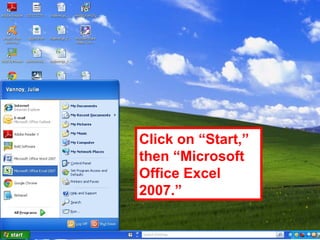
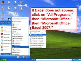
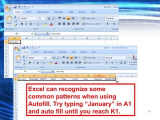
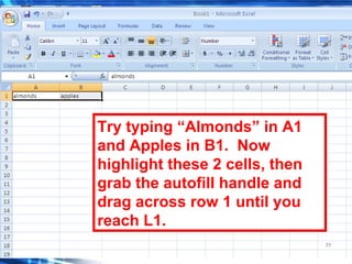
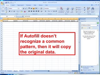
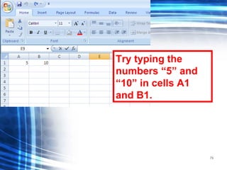
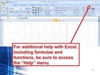
1. This document provides instructions for using basic Microsoft Excel functions like opening Excel, navigating the ribbon interface, entering data into cells, formatting cells, using autofill, and other common tasks.
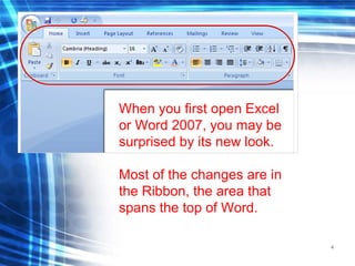
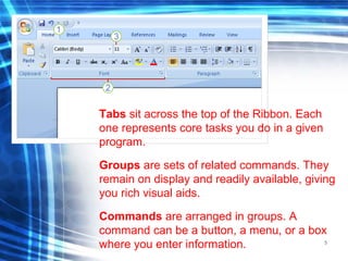
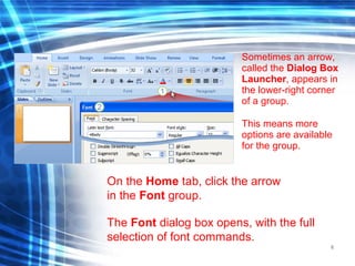
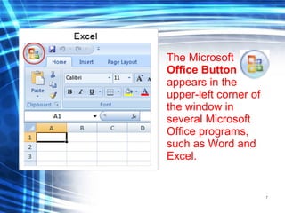
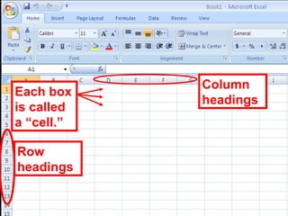
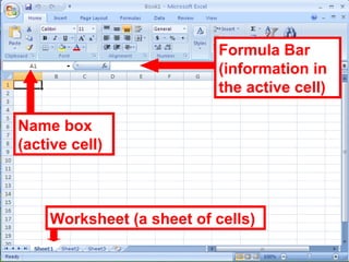
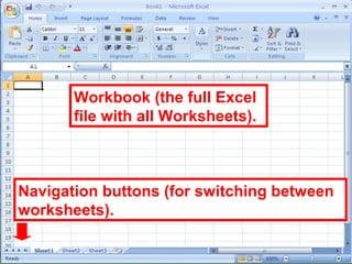
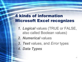
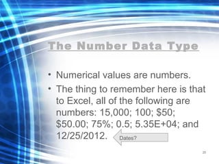
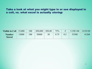
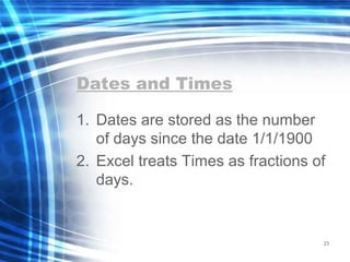
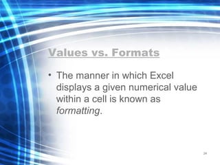
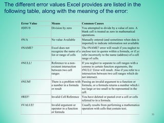
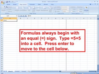
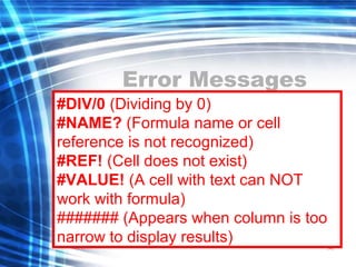
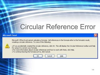
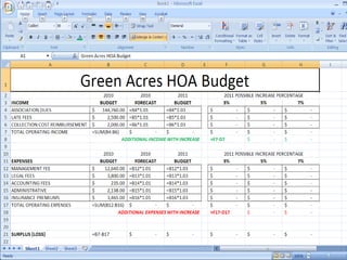
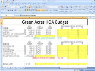
2. It explains the different parts of the Excel interface like tabs, groups, commands, and describes the different data types Excel recognizes.
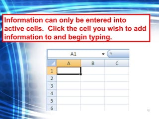
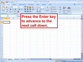
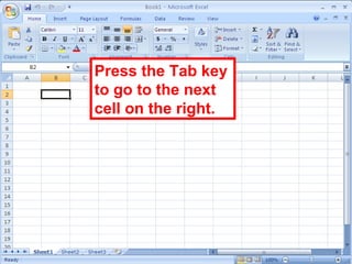
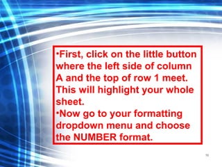
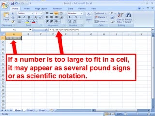
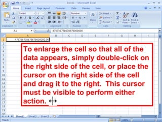
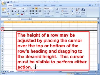
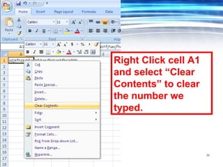
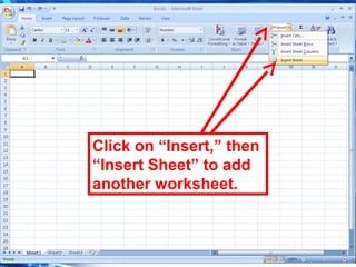
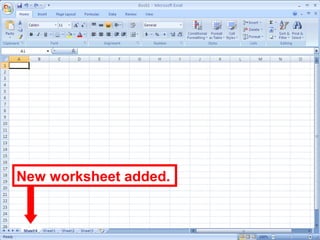
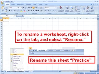
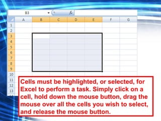
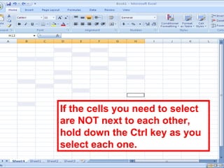
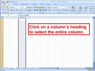
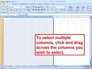
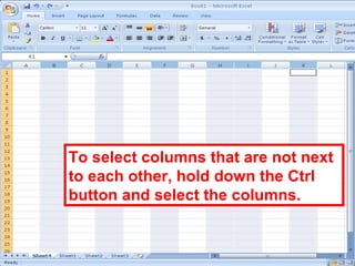
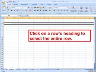
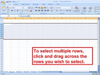
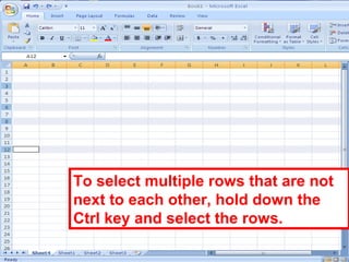
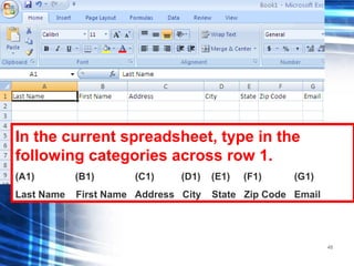
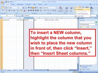
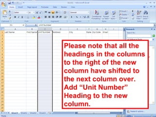
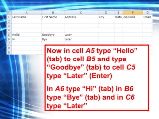
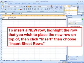
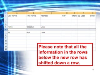
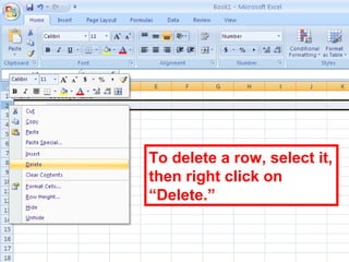
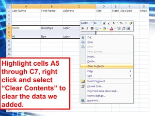
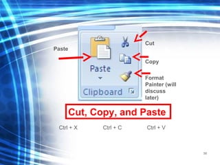
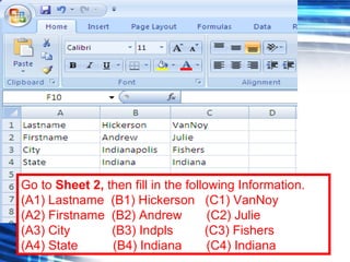
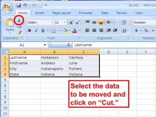
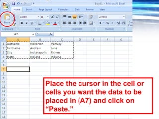
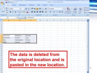
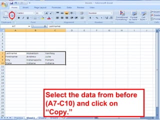
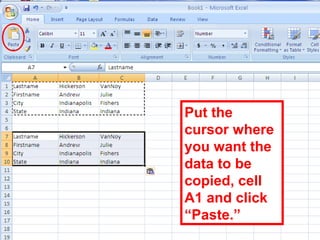
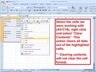
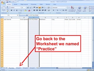
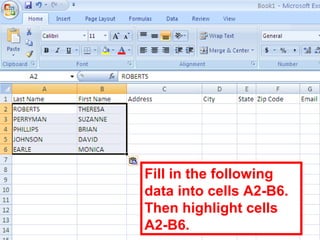
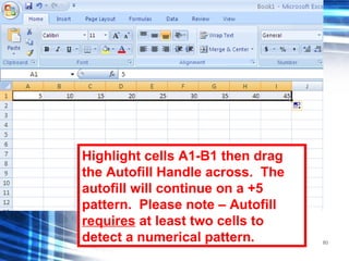
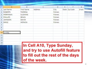
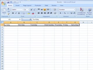
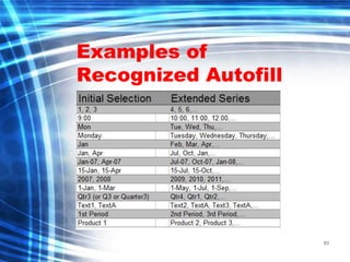
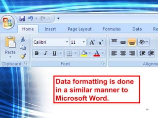
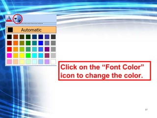
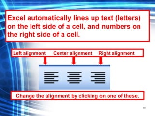
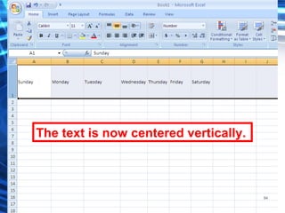
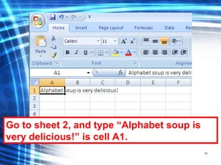
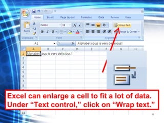
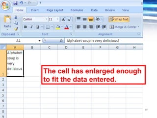
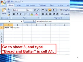
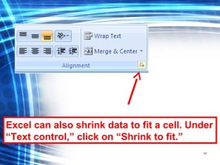
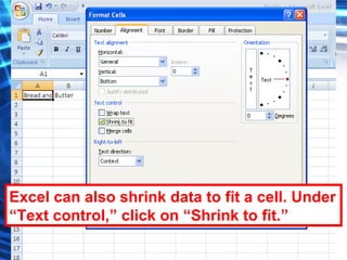
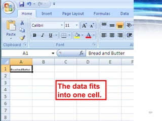
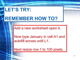
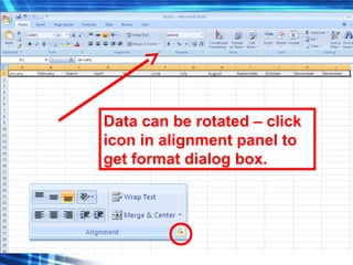
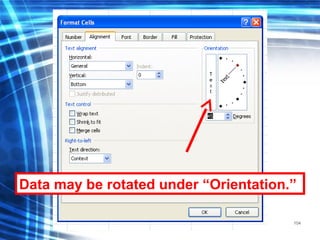
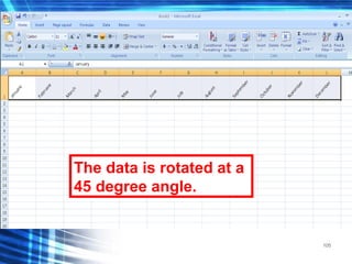
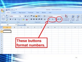
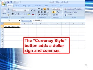
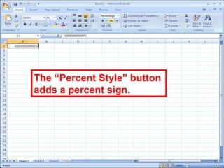
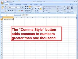
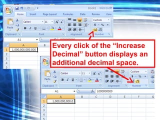
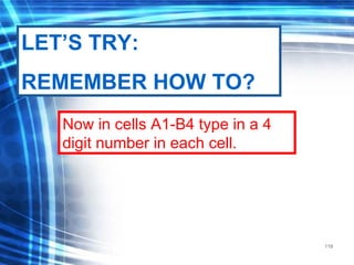
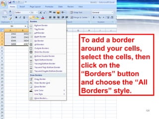
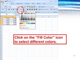
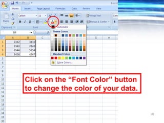
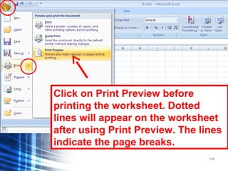
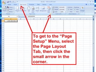
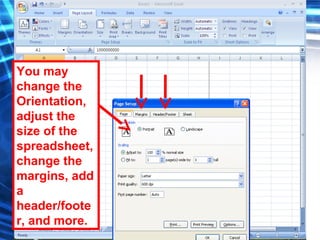
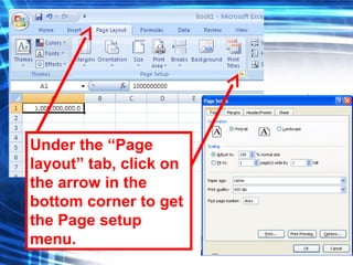
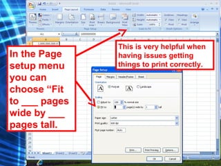
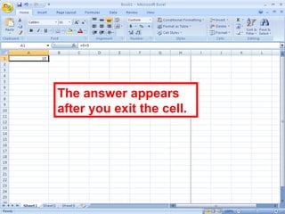
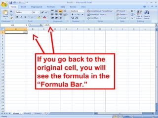
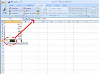
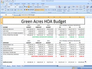
3. The document provides step-by-step examples for tasks like entering text and numbers, selecting cells, cutting/copying/pasting data, inserting and deleting rows and columns, and using basic formatting options.