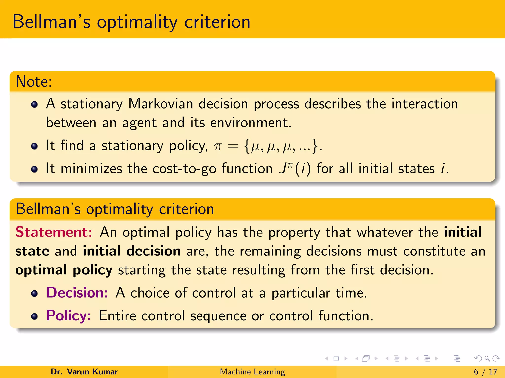
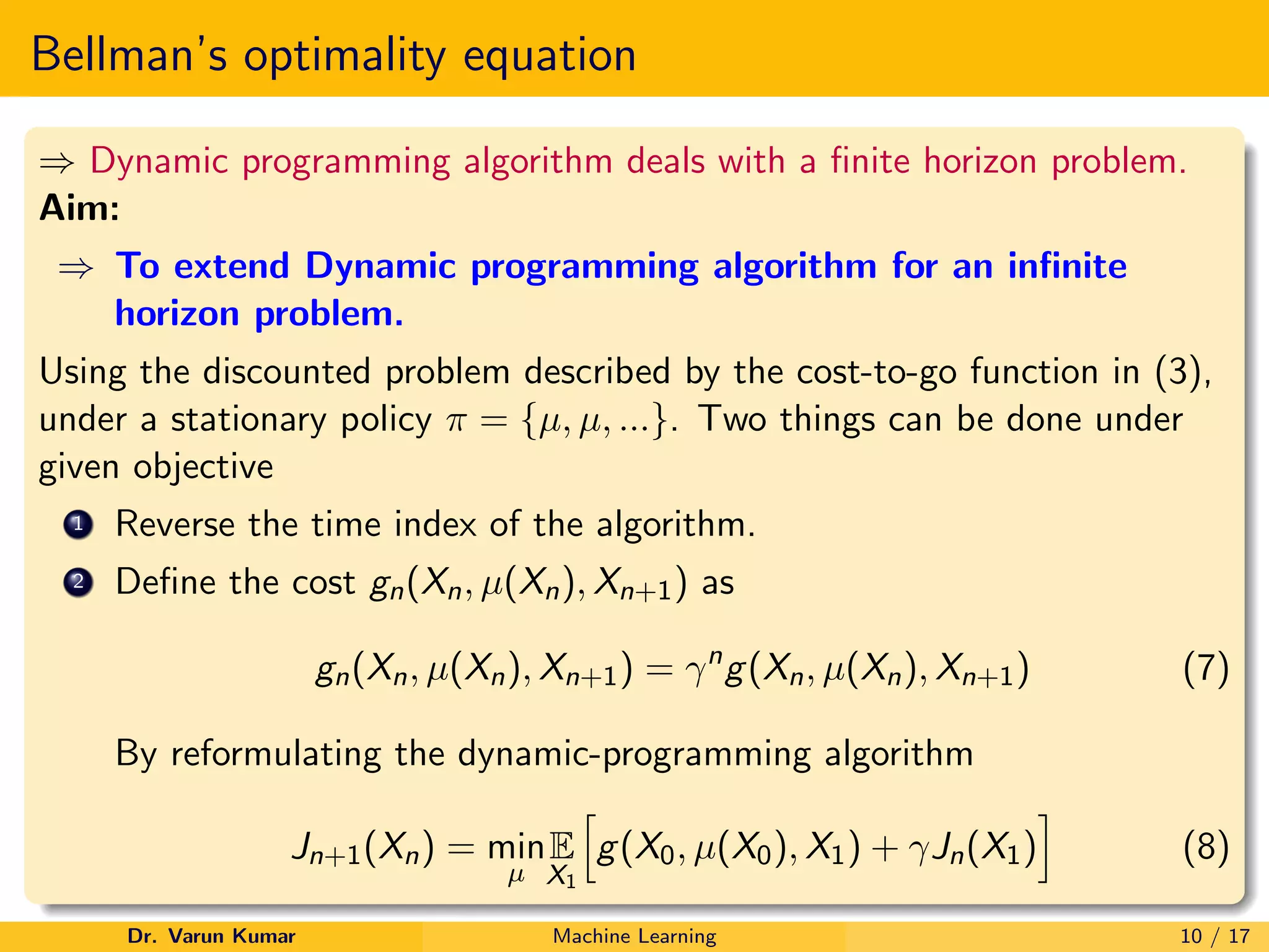
1. Bellman's optimality criterion states that the optimal policy for the remaining decisions must constitute an optimal policy starting from the state resulting from the first decision. 2. Bellman's optimality equation extends dynamic programming to infinite horizon problems by defining the cost at each time step as a discounted value and formulating the optimal cost as the minimum expected immediate cost plus the discounted expected future cost. 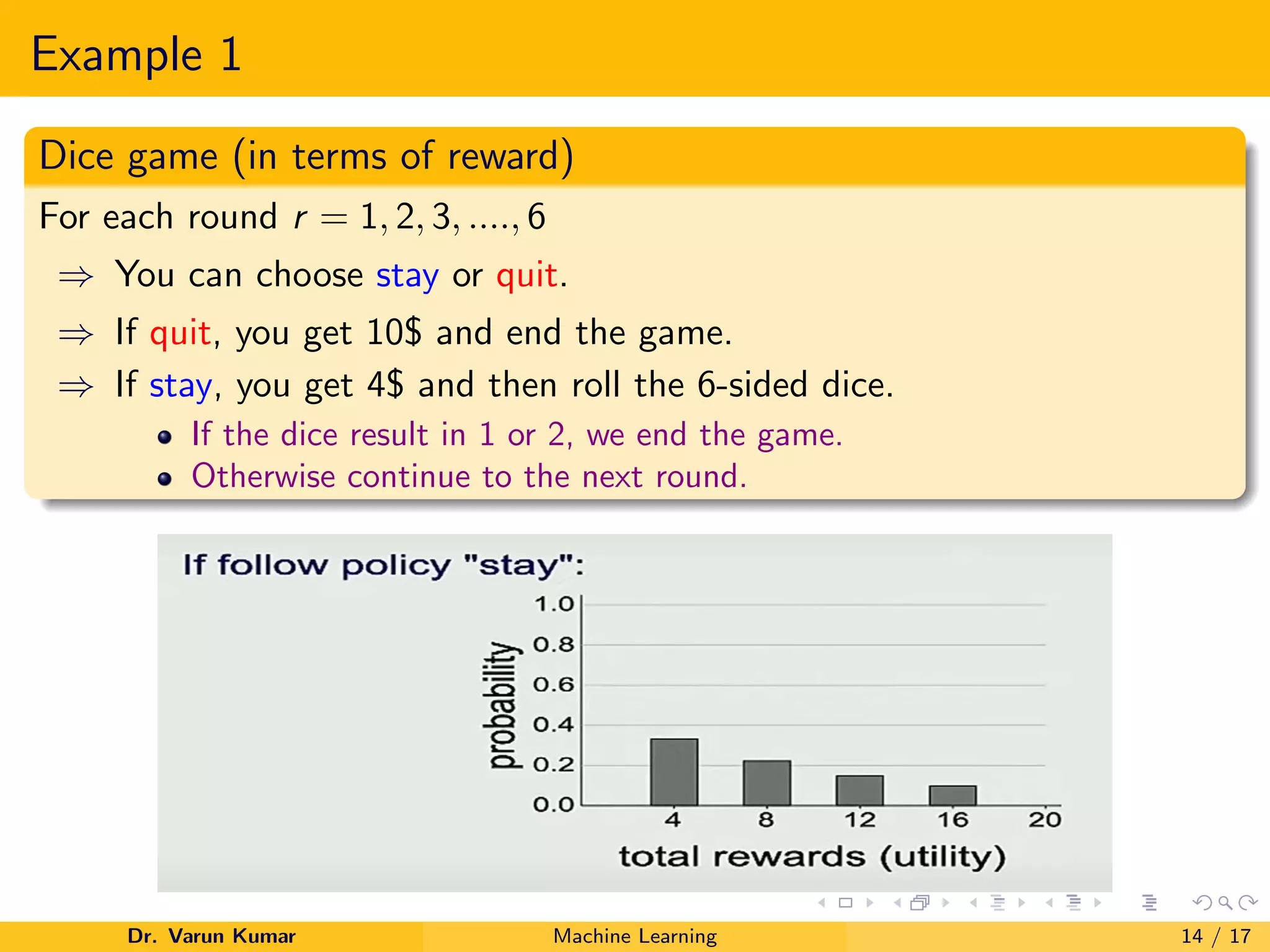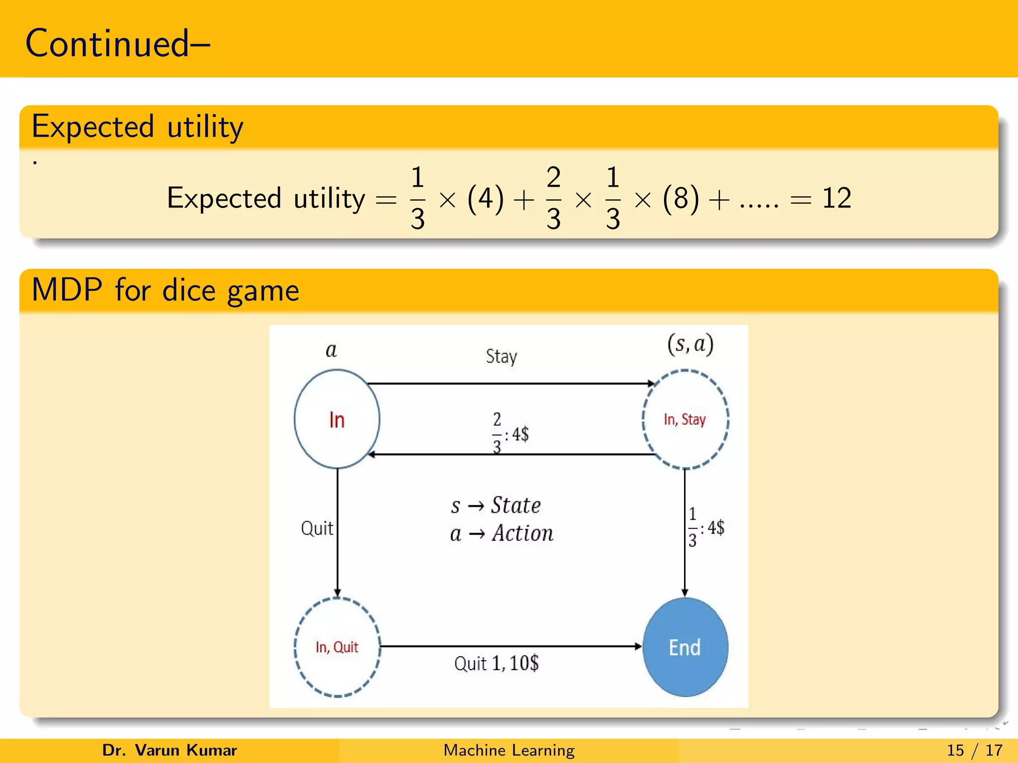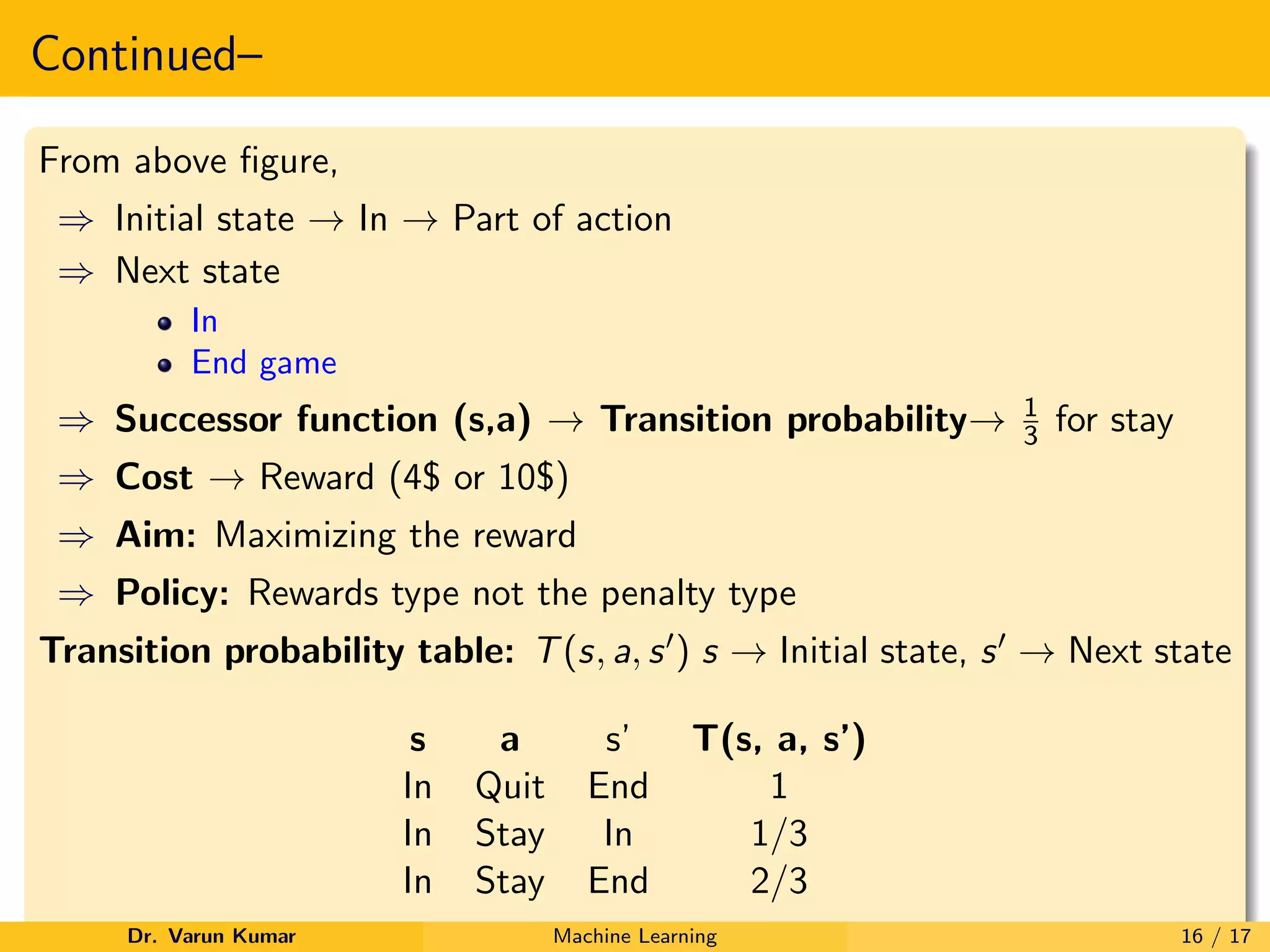3. An example of a dice game Markov decision process is presented to illustrate calculating expected rewards and transition probabilities to determine the optimal policy using Bellman's optimality equation.

1. Role of Bellman’s Equation in Reinforcement Learning
Dr. Varun Kumar
Dr. Varun Kumar Machine Learning 1 / 17

2. Outlines
1 Policy in Reinforcement Learning
2 Basic Problem
3 Bellman’s Optimality Criterion
4 Dynamic Programming Algorithm
5 Bellman’s Optimality Equation
6 Example
7 References
Dr. Varun Kumar Machine Learning 2 / 17

3. Policy in Reinforcement Learning
Brief about reinforcement learning
⇒ At each transition from one state to another, a cost is incurred by the
agent.
⇒ At nth transition from state i to state j under action aik, the agent
incurs a cost denoted by
Cost = γn
g(i, aik, j) (1)
♦ g(., ., .) → Prescribed function
♦ γ → Discount factor, 0 ≤ γ < 1
⇒ In reinforcement learning, there is a need proper policy, i.e mapping of
state of action.
⇒ Policy: It is a rule used by the agent to decide what to do, given
knowledge of the current state of the environment. It is denoted as
π = {µ0, µ1, µ2...} (2)
Dr. Varun Kumar Machine Learning 3 / 17

4. Continued–
where µn is a function that maps the state Xn = i into an action
An = a at time-step n = 0, 1, 2, ... This mapping is such that
µn(i) ∈ Ai For all states i ∈ X
Ai → Set of all possible action taken by agent in state i.
Types of policy:
Non-stationary → Time varying → π = {µ0, µ1, µ2...}
Stationary → Time invariant → π = {µ, µ, µ...}
⇒ Stationary policy specifies exactly the same action each time a
particular state is visited.
⇒ For a stationary policy, Markov chain may be stationary or
non-stationary.
.
Dr. Varun Kumar Machine Learning 4 / 17

5. Basic problem in dynamic programming
Infinite horizon problem
⇒ In an infinite-horizon problem, the cost accumulates over a infinite
number of stages.
⇒ Infinite-horizon problem provides a reasonable approximation, but
there is a need for high number of stages.
⇒ Let g Xn, µn(Xn), Xn+1
is a observed cost incurred as a result of a
transition from state Xn to state Xn+1 under the action of policy
µn(Xn). The total expected cost in an infinite horizon problem,
Jπ
(i) = E
h ∞
X
n=0
γn
g Xn, µn(Xn), Xn+1
|X0 = i
i
(3)
Jπ
(i) → Cost-to-go function
γ → Discount factor
Starting state X0 = i
,
Dr. Varun Kumar Machine Learning 5 / 17

6. Bellman’s optimality criterion
Note:
A stationary Markovian decision process describes the interaction
between an agent and its environment.
It find a stationary policy, π = {µ, µ, µ, ...}.
It minimizes the cost-to-go function Jπ(i) for all initial states i.
Bellman’s optimality criterion
Statement: An optimal policy has the property that whatever the initial
state and initial decision are, the remaining decisions must constitute an
optimal policy starting the state resulting from the first decision.
Decision: A choice of control at a particular time.
Policy: Entire control sequence or control function.
Dr. Varun Kumar Machine Learning 6 / 17

7. Finite horizon
A finite horizon problem for which the cost-to-go function is defined as
J0(X0) = E
h
gK (XK ) +
K−1
X
n=0
gn Xn, µn(Xn), Xn+1
i
(4)
1 K is the planning horizon (number of stages)
2 gK (XK ) is the terminal cost
3 X0 is the expectation wrt the remaining states X1, X2, ...
Optimal policy
⇒ Let π∗ = {µ∗
0, µ∗
1, ..., µ∗
K−1} be an optimal policy for the finite horizon.
⇒ Consider a sub-problem where the environment is in state Xn at time
n and we want to minimize the cost-to-go function Jn(Xn).
Dr. Varun Kumar Machine Learning 7 / 17

8. Continued–
Jn(Xn) = E
h
gK (Xk) +
K−1
X
k=n
gn Xk, µk(Xk), Xk+1
i
(5)
for n = 0, 1, ...., K − 1. Here truncated policy π∗ = {µ∗
n, µ∗
n+1, ...., µ∗
K−1}
will be optimal for the sub-problem.
Dr. Varun Kumar Machine Learning 8 / 17

9. Dynamic-programming algorithm
Dynamic-programming algorithm proceeds backward in time from N − 1 to 0.
Let π = {µ0, µ1, ..., µK−1} denotes the permissible policy.
For each n = 0, 1, ...K − 1, let πn = {µn, µn+1, ..., µK−1}
J∗
n (Xn) is the optimal cost for the (K − n) stages.
Problem starts at state Xn at time n and ends at time K
J∗
n (Xn) = min
πn
E
(Xn+1,...XK−1)
h
gK (XK ) +
K−1
X
k=n
gk(Xk, µk(Xk), Xk+1)
i
= min
µn
E
Xn+1
h
gn(Xn, µn(Xn), Xn+1) + J∗
n+1(Xn+1)
i
(6)
Dr. Varun Kumar Machine Learning 9 / 17

10. Bellman’s optimality equation
⇒ Dynamic programming algorithm deals with a finite horizon problem.
Aim:
⇒ To extend Dynamic programming algorithm for an infinite
horizon problem.
Using the discounted problem described by the cost-to-go function in (3),
under a stationary policy π = {µ, µ, ...}. Two things can be done under
given objective
1 Reverse the time index of the algorithm.
2 Define the cost gn(Xn, µ(Xn), Xn+1) as
gn(Xn, µ(Xn), Xn+1) = γn
g(Xn, µ(Xn), Xn+1) (7)
By reformulating the dynamic-programming algorithm
Jn+1(Xn) = min
µ
E
X1
h
g(X0, µ(X0), X1) + γJn(X1)
i
(8)
Dr. Varun Kumar Machine Learning 10 / 17

11. Continued–
Let J∗(i) denotes the optimal infinite horizon cost for the initial state
X0 = i then mathematically it can be expressed as
J∗
(i) = lim
K→∞
JK (i) (9)
For expressing the optimal infinite horizon cost J∗(i), we proceed in two
stages.
1 Evaluate the expectation of the cost g(i, µ(i), X1) wrt X1. Hence,
E[g(i), µ(i), X1] =
N
X
j=1
pij g(i, µ(i), j) (10)
(a) N → Number of states of the environment.
(b) pij → Transition probability from state X0 = i to X1 = j.
Dr. Varun Kumar Machine Learning 11 / 17

12. Continued–
The quantity defined in (10) is the immediate expected cost incurred at
state i by the action recommended by the policy µ. This cost is denoted
by c(i, µ(i))
c(i, µ(i)) =
N
X
j=1
pij g(i, µ(i), j) (11)
E[J∗
(X1)] =
N
X
j=1
pij J∗
(j) (12)
J∗
(i) = min
µ
c(i, µ(i)) + γ
N
X
j=1
pij (µ)J∗
(j)
(13)
Dr. Varun Kumar Machine Learning 12 / 17

13. Policy iteration
content...
Dr. Varun Kumar Machine Learning 13 / 17

14. Example 1
Dice game (in terms of reward)
For each round r = 1, 2, 3, ...., 6
⇒ You can choose stay or quit.
⇒ If quit, you get 10$ and end the game.
⇒ If stay, you get 4$ and then roll the 6-sided dice.
If the dice result in 1 or 2, we end the game.
Otherwise continue to the next round.
Dr. Varun Kumar Machine Learning 14 / 17

15. Continued–
Expected utility
.
Expected utility =
1
3
× (4) +
2
3
×
1
3
× (8) + ..... = 12
MDP for dice game
Dr. Varun Kumar Machine Learning 15 / 17

16. Continued–
From above figure,
⇒ Initial state → In → Part of action
⇒ Next state
In
End game
⇒ Successor function (s,a) → Transition probability→ 1
3 for stay
⇒ Cost → Reward (4$ or 10$)
⇒ Aim: Maximizing the reward
⇒ Policy: Rewards type not the penalty type
Transition probability table: T(s, a, s0) s → Initial state, s0 → Next state
s a s’ T(s, a, s’)
In Quit End 1
In Stay In 1/3
In Stay End 2/3
Dr. Varun Kumar Machine Learning 16 / 17

17. References
E. Alpaydin, Introduction to machine learning. MIT press, 2020.
T. M. Mitchell, The discipline of machine learning. Carnegie Mellon University,
School of Computer Science, Machine Learning , 2006, vol. 9.
J. Grus, Data science from scratch: first principles with python. O’Reilly Media,
2019.
Dr. Varun Kumar Machine Learning 17 / 17