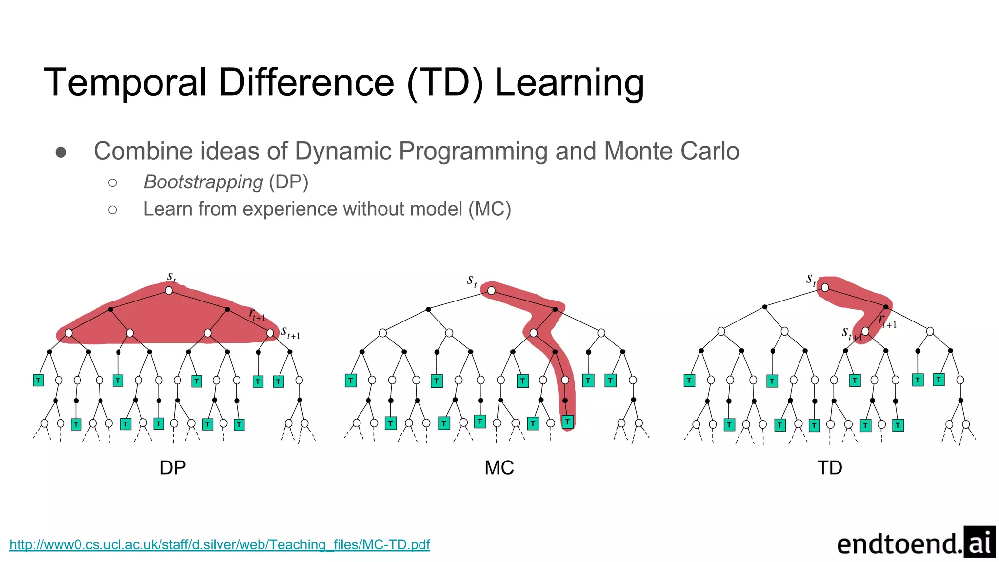
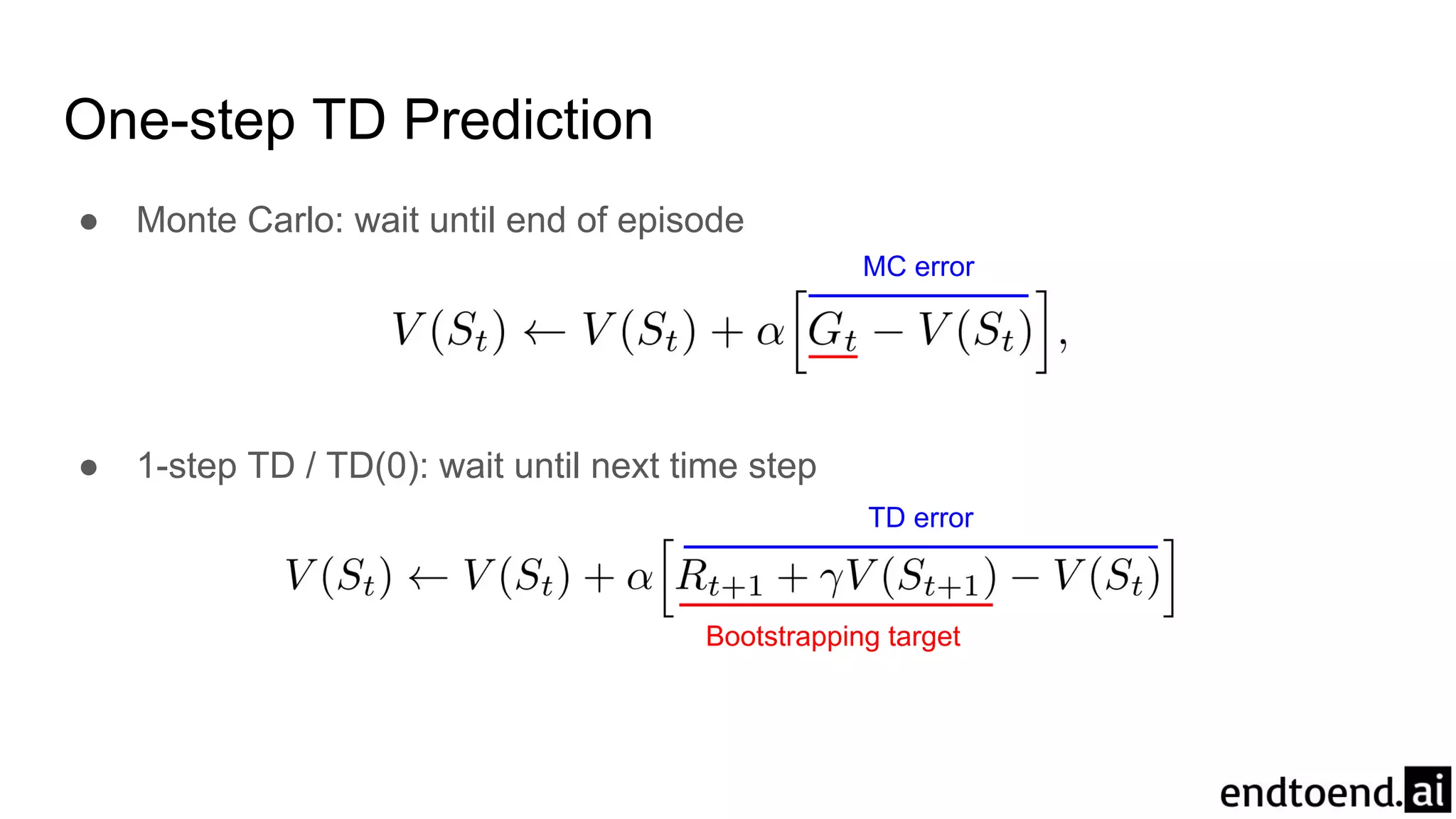
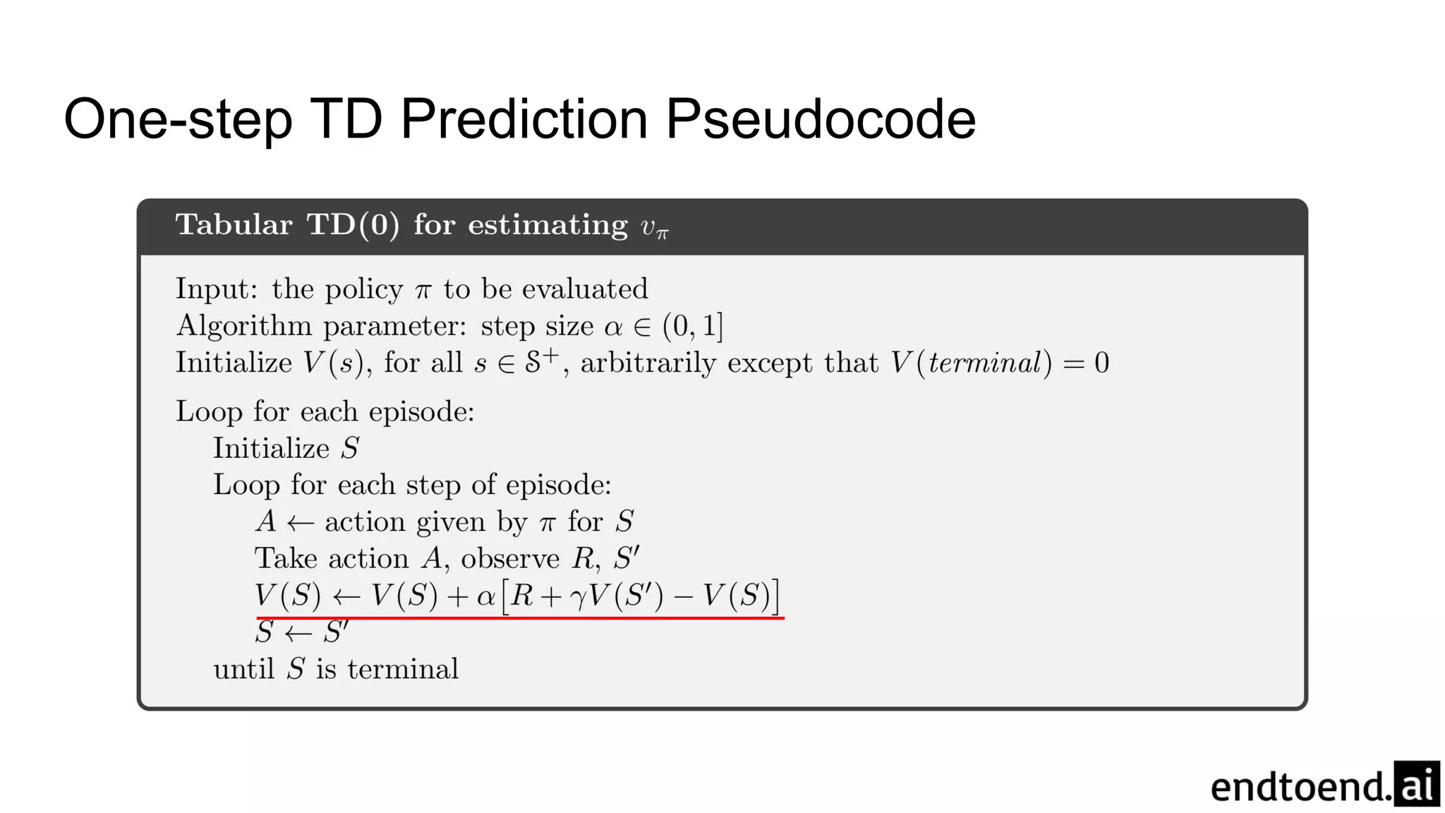
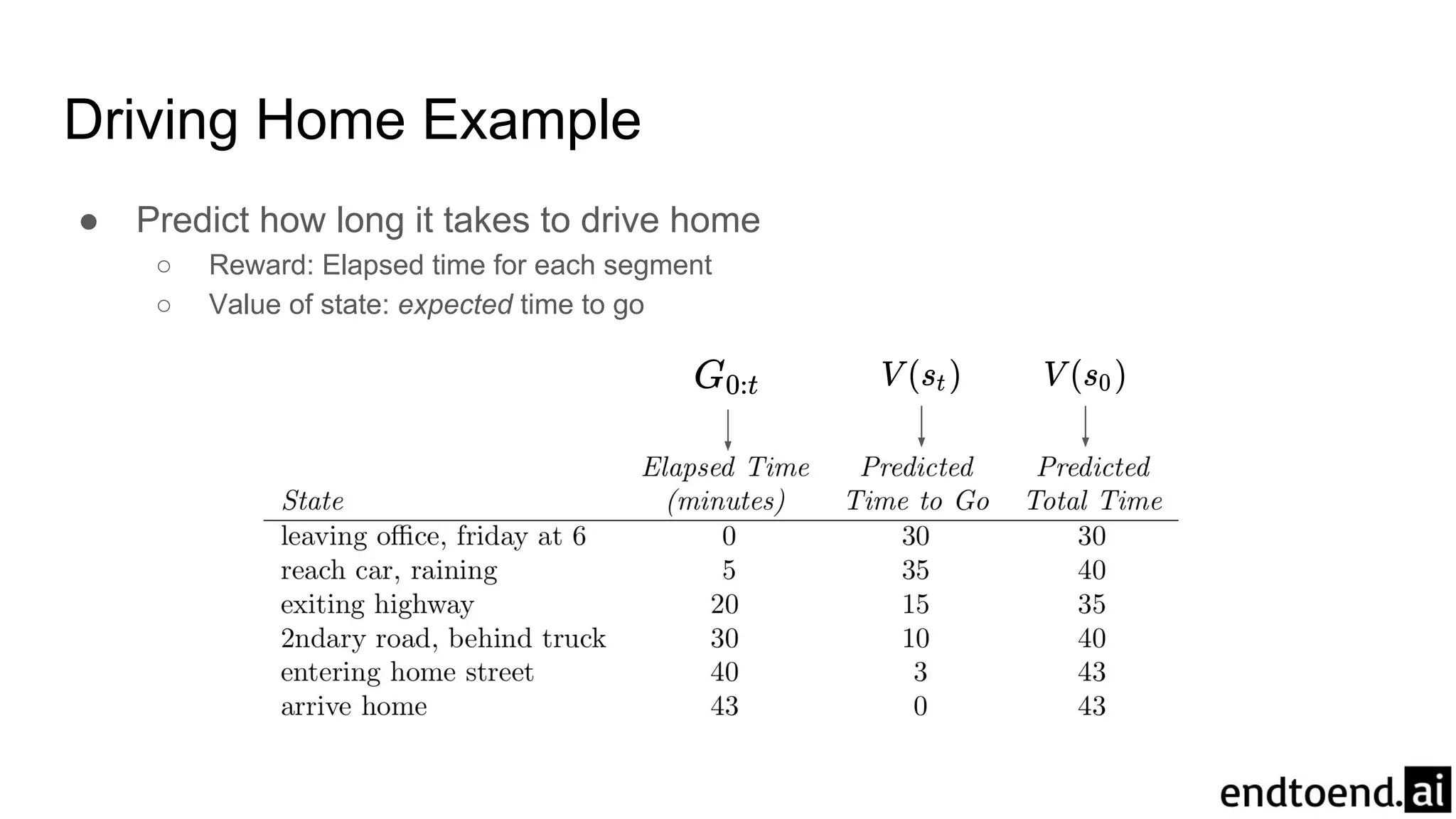
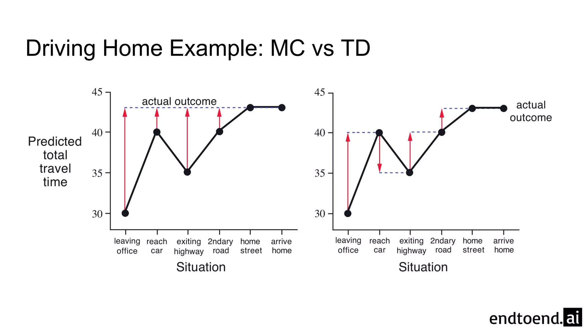
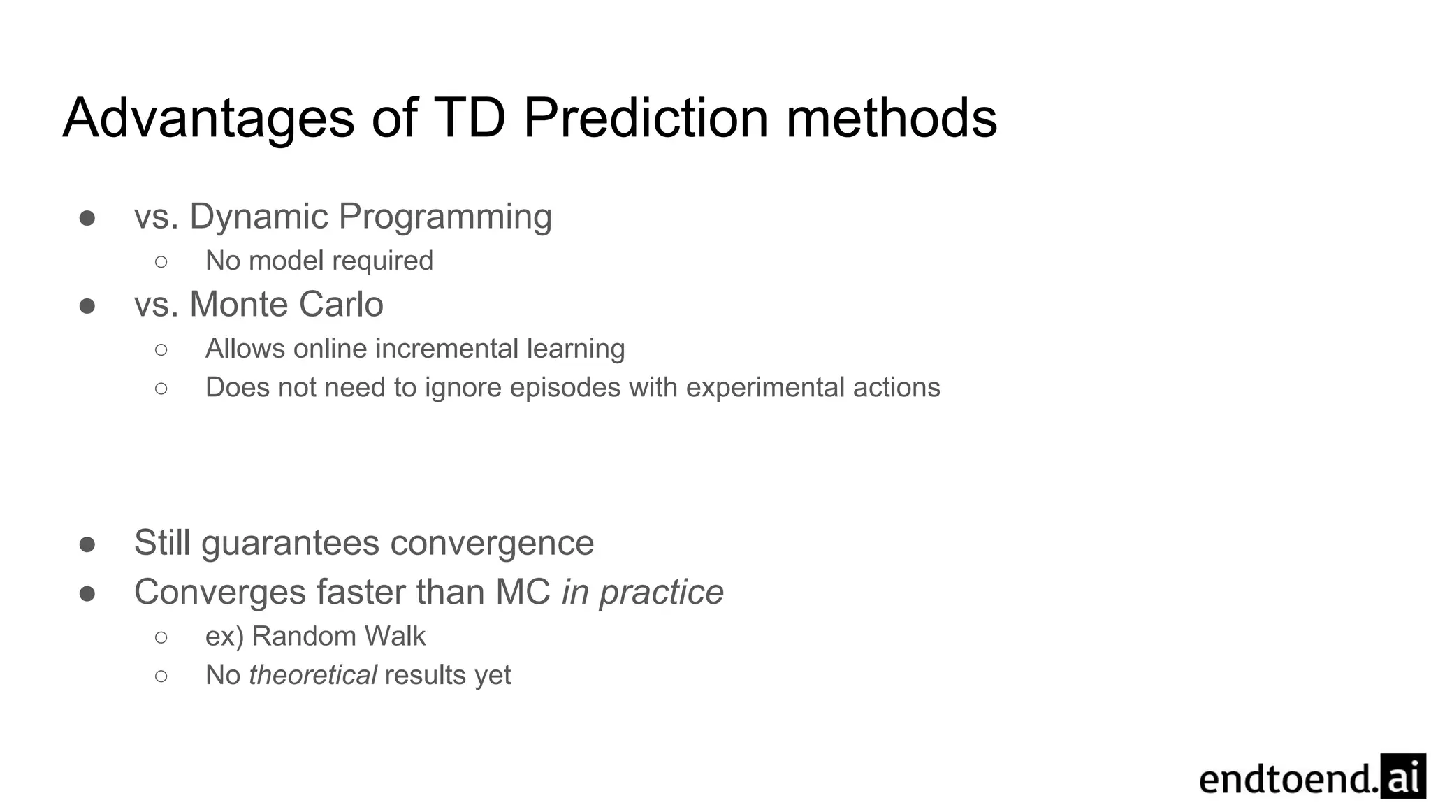
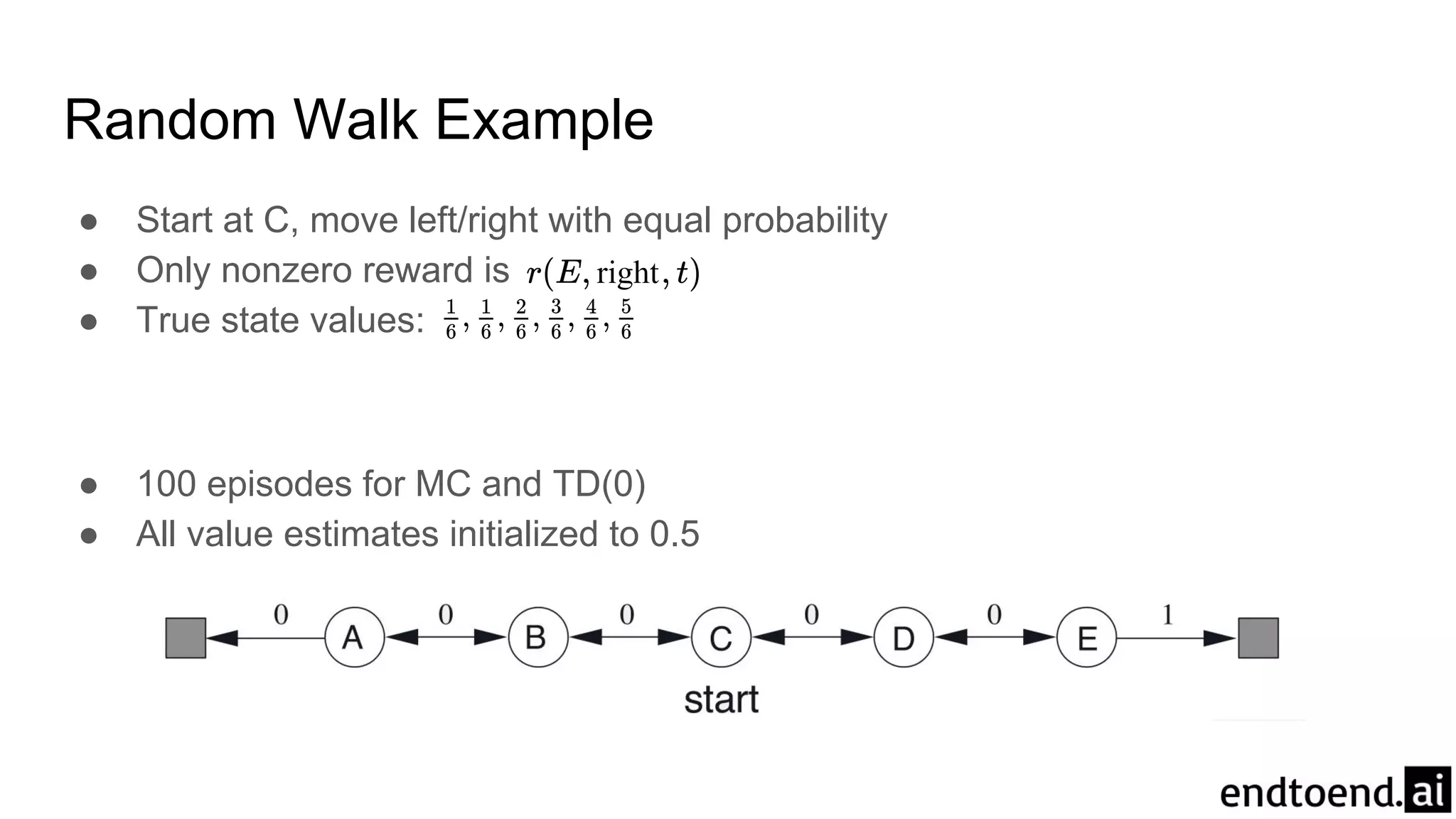
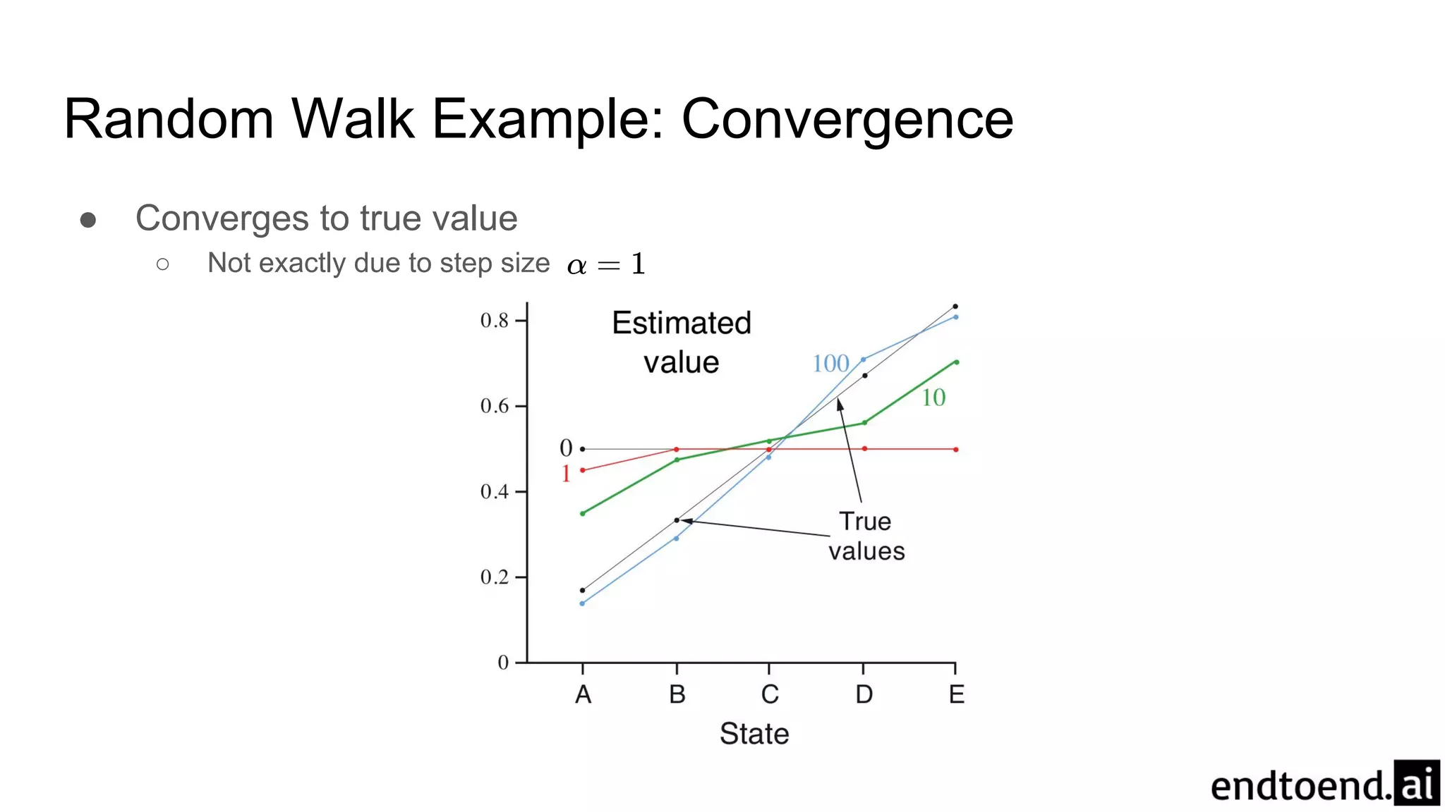
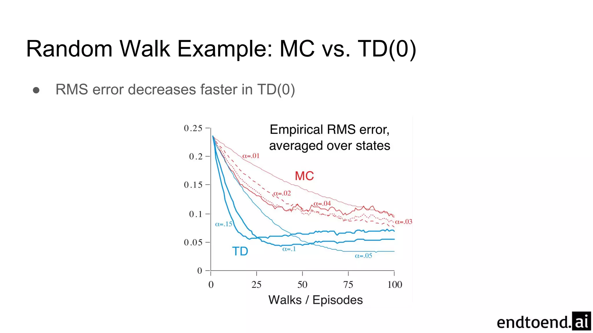
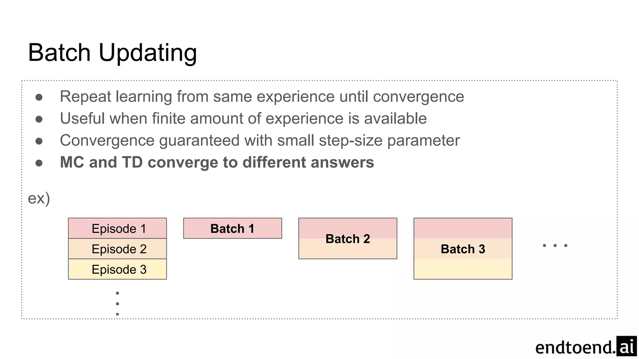
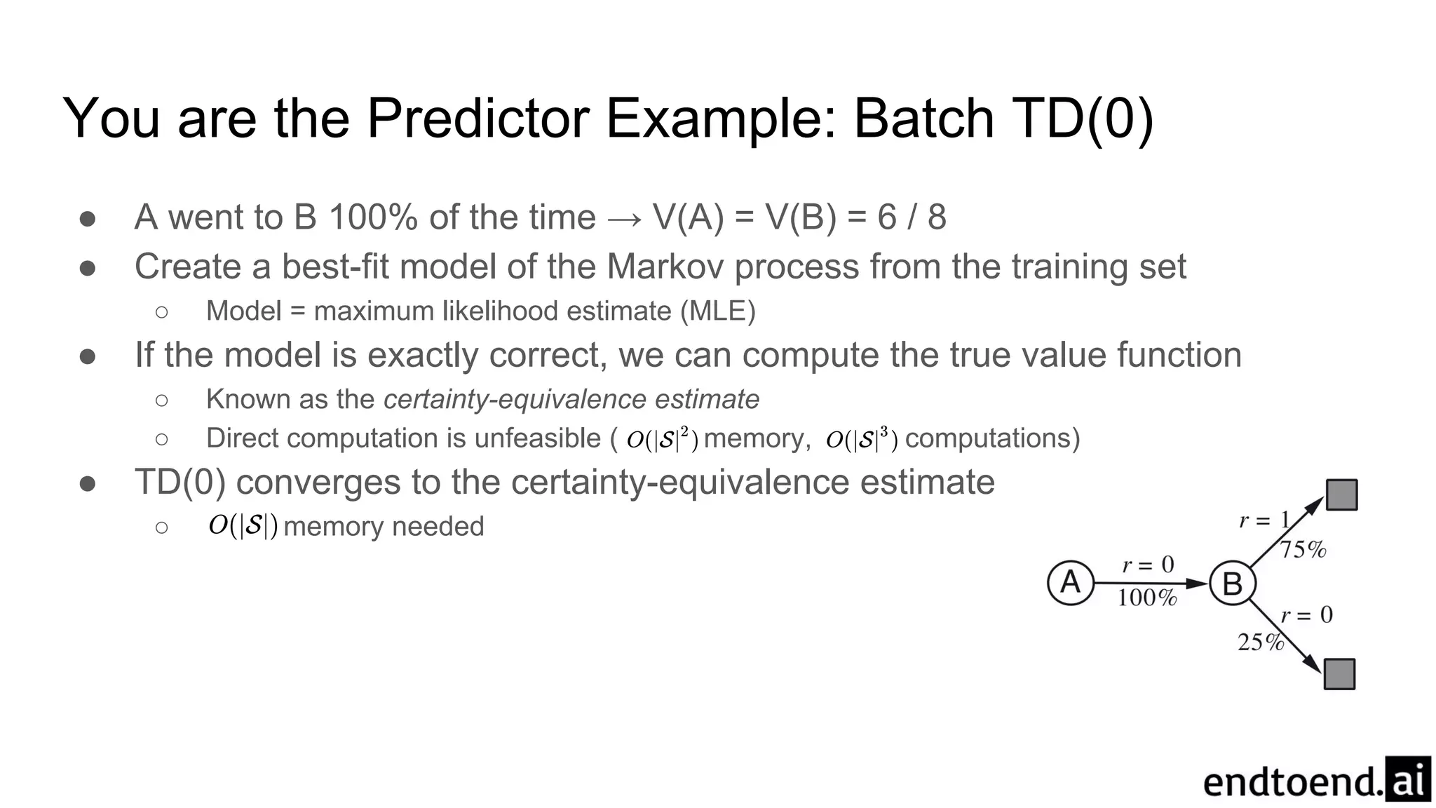
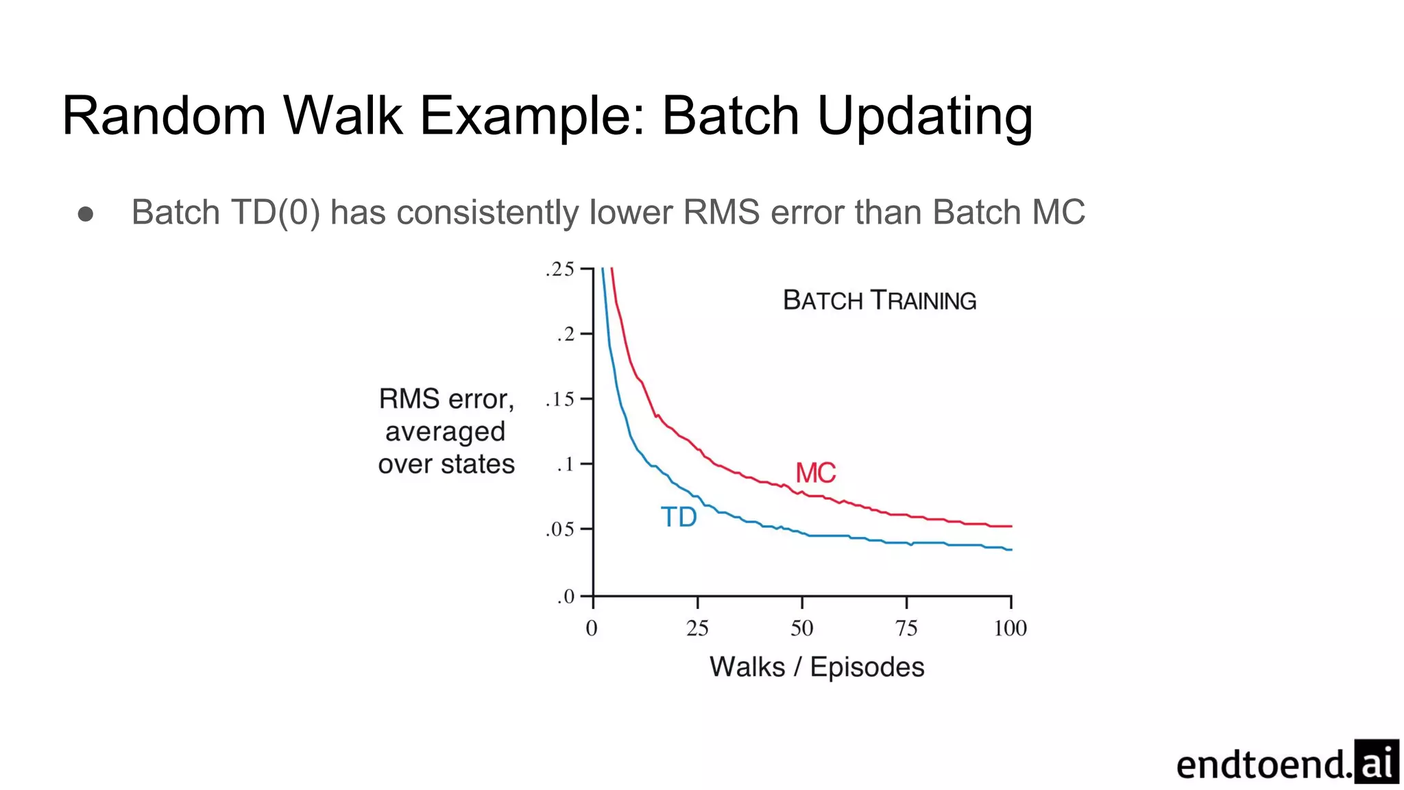
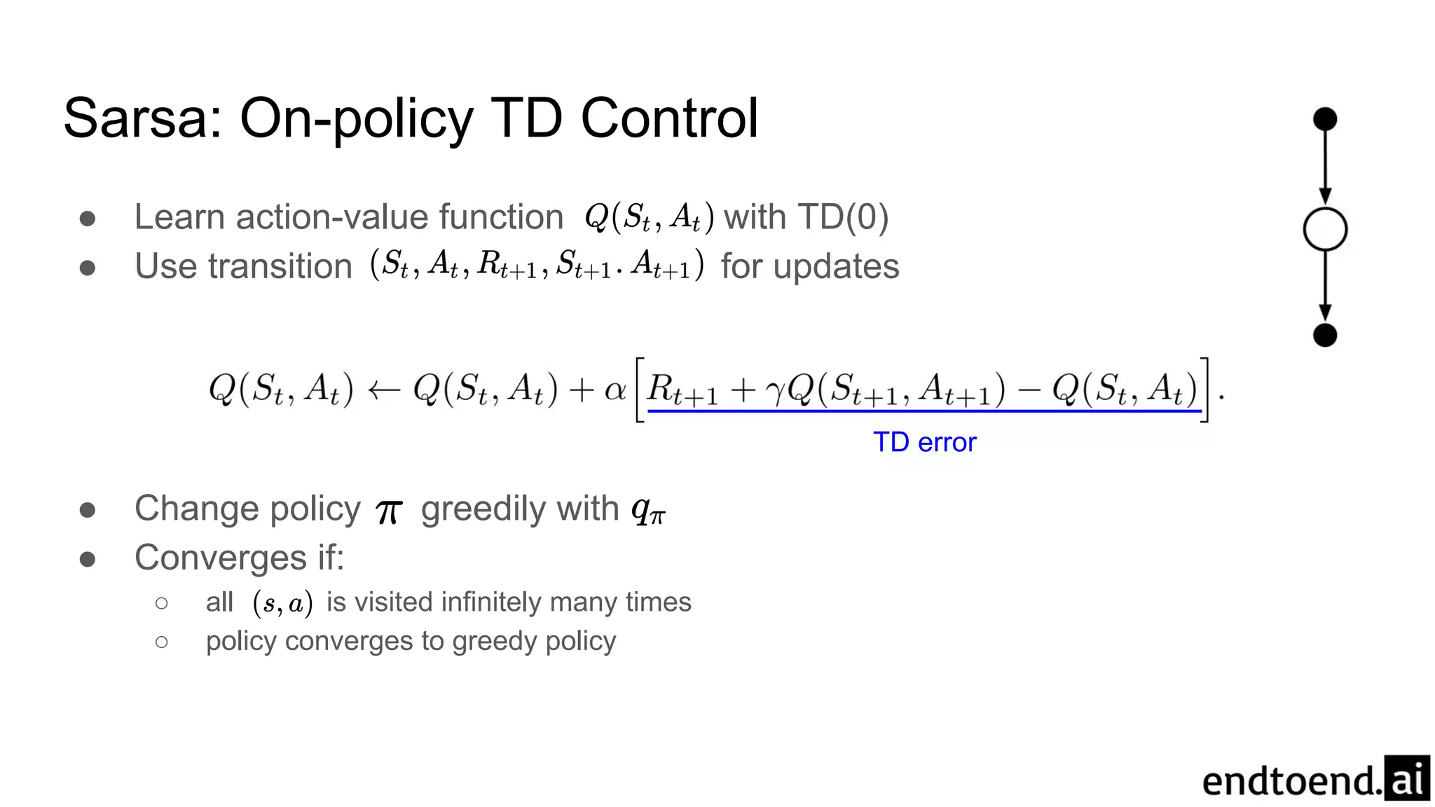
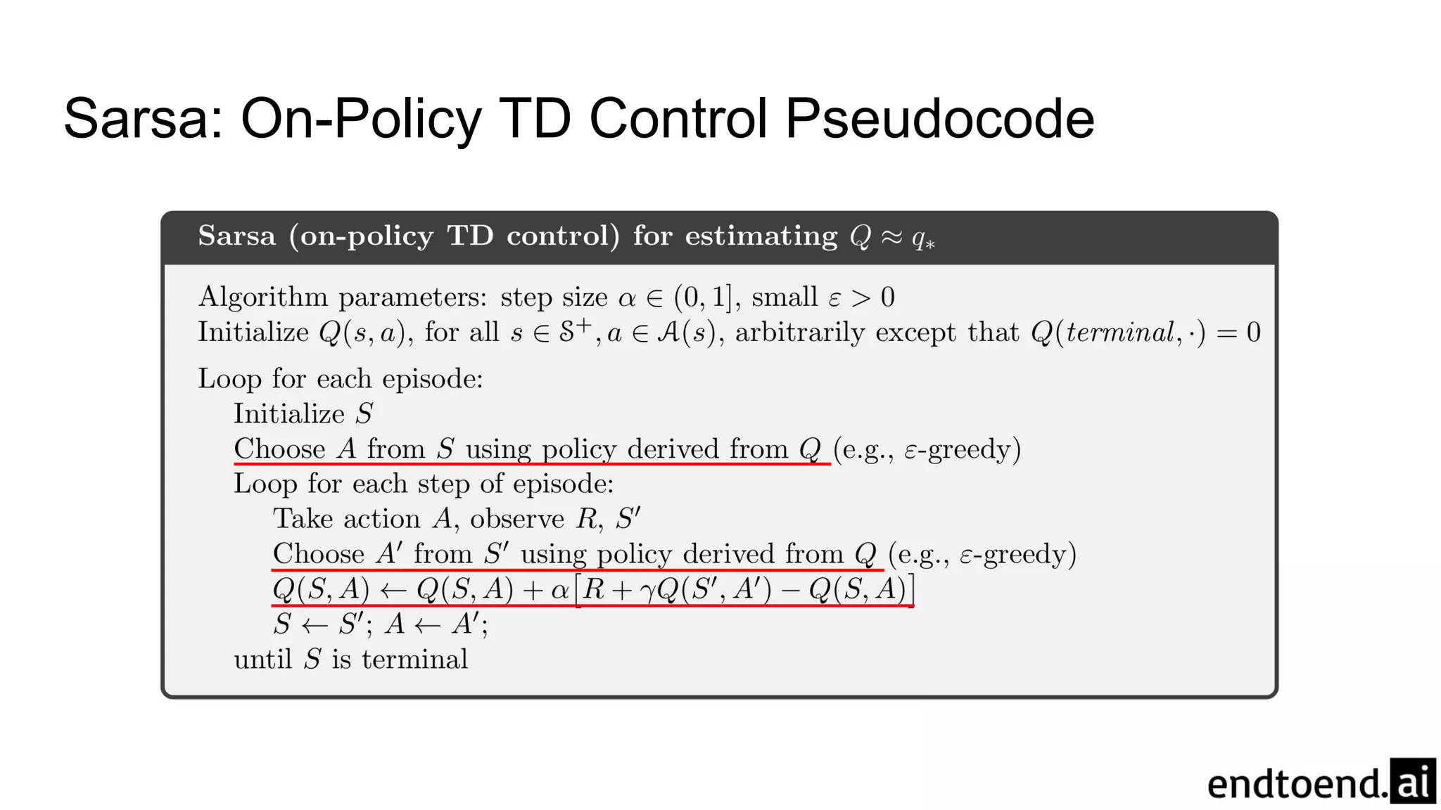
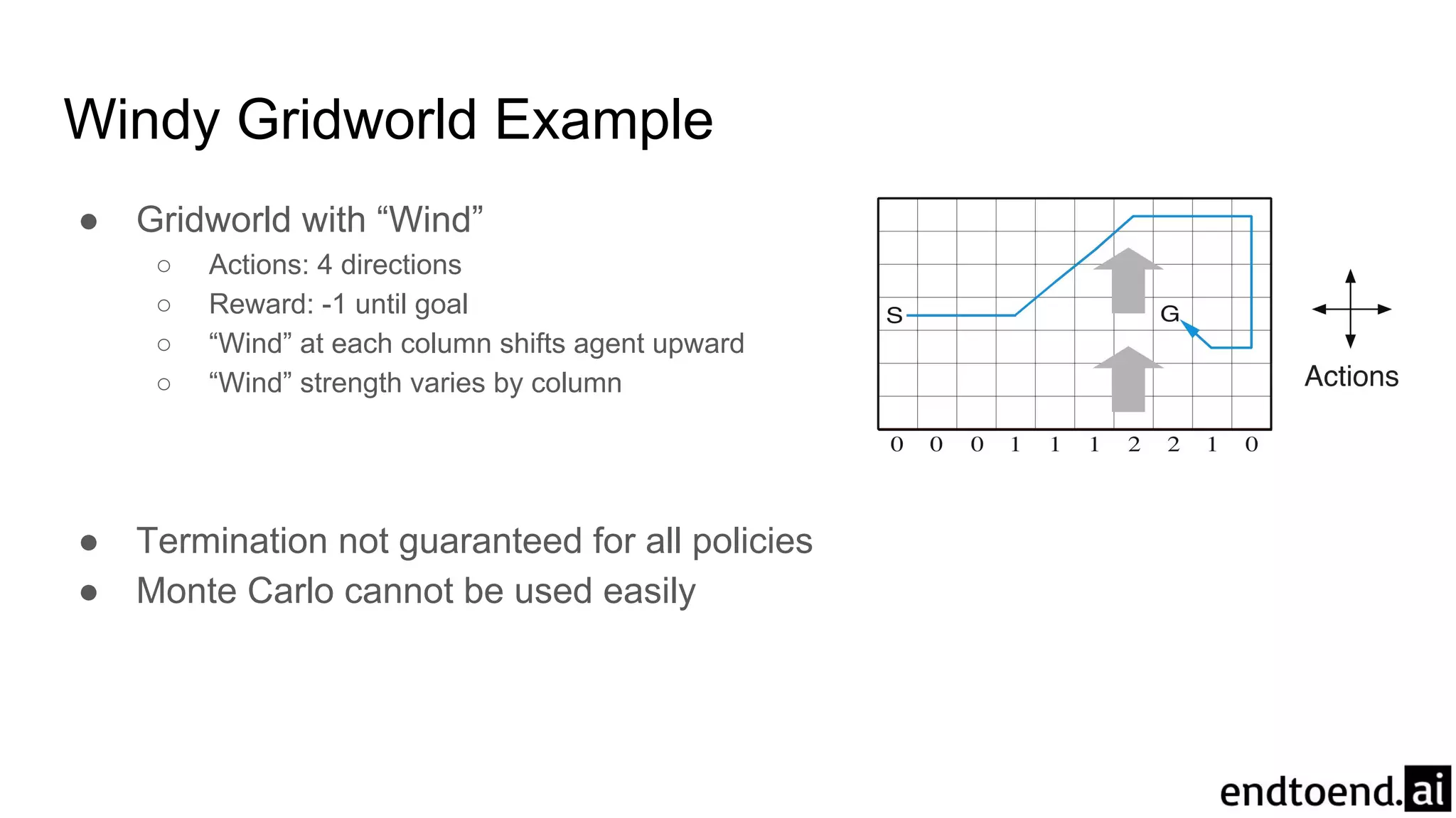
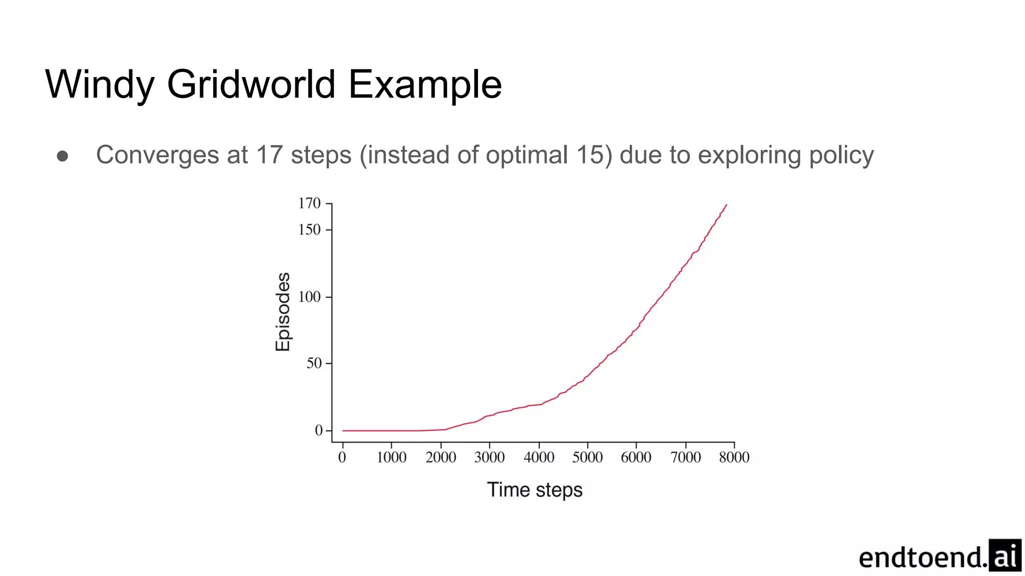
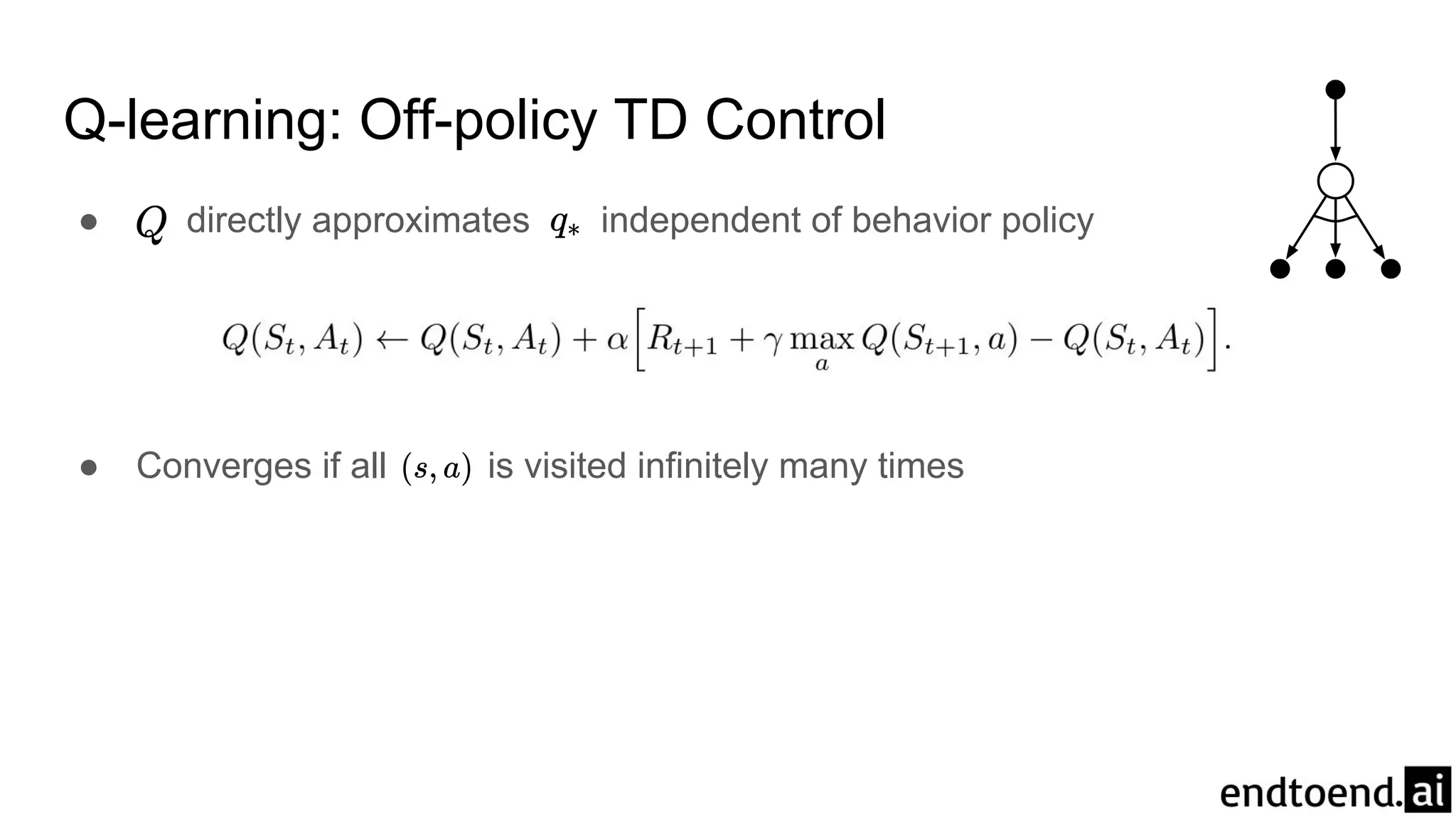
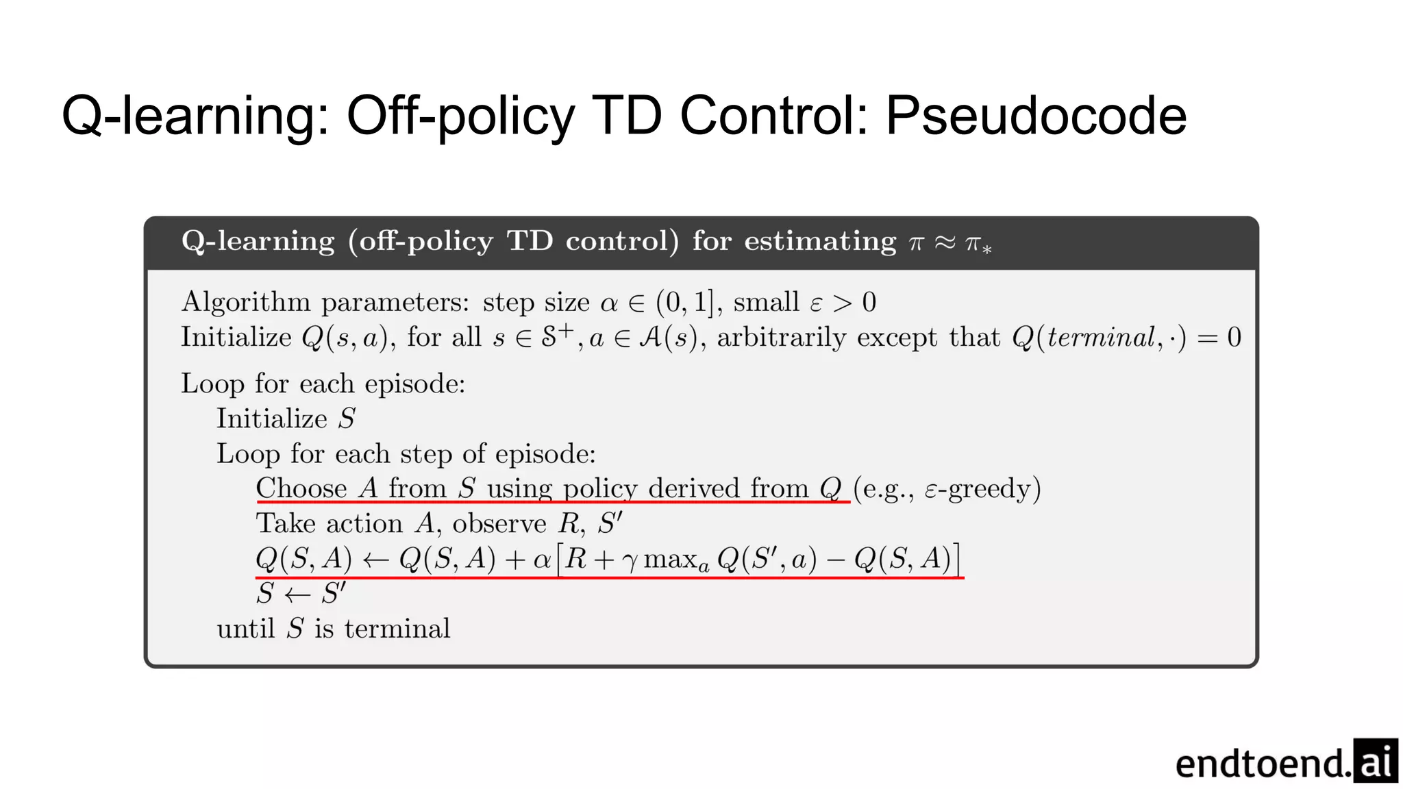
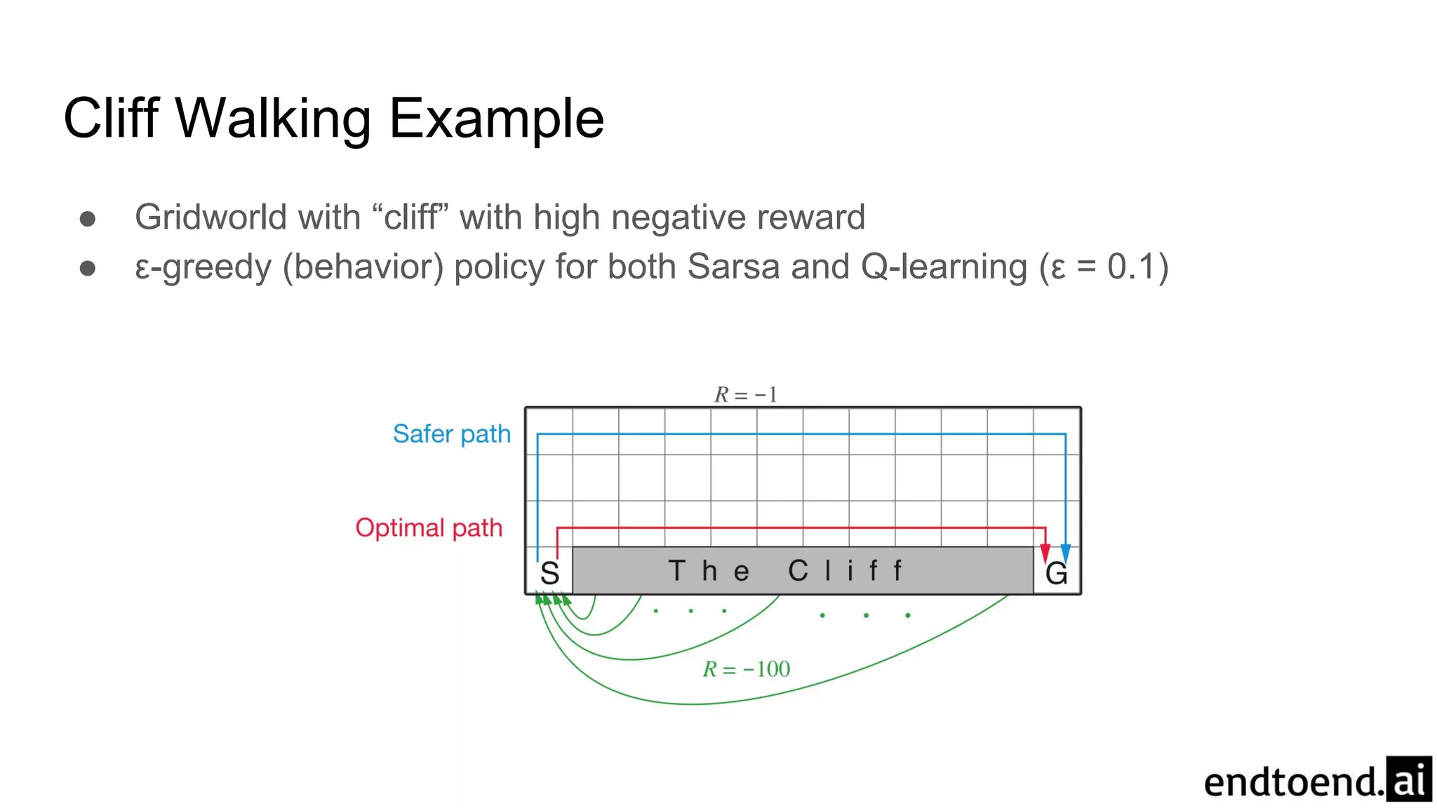
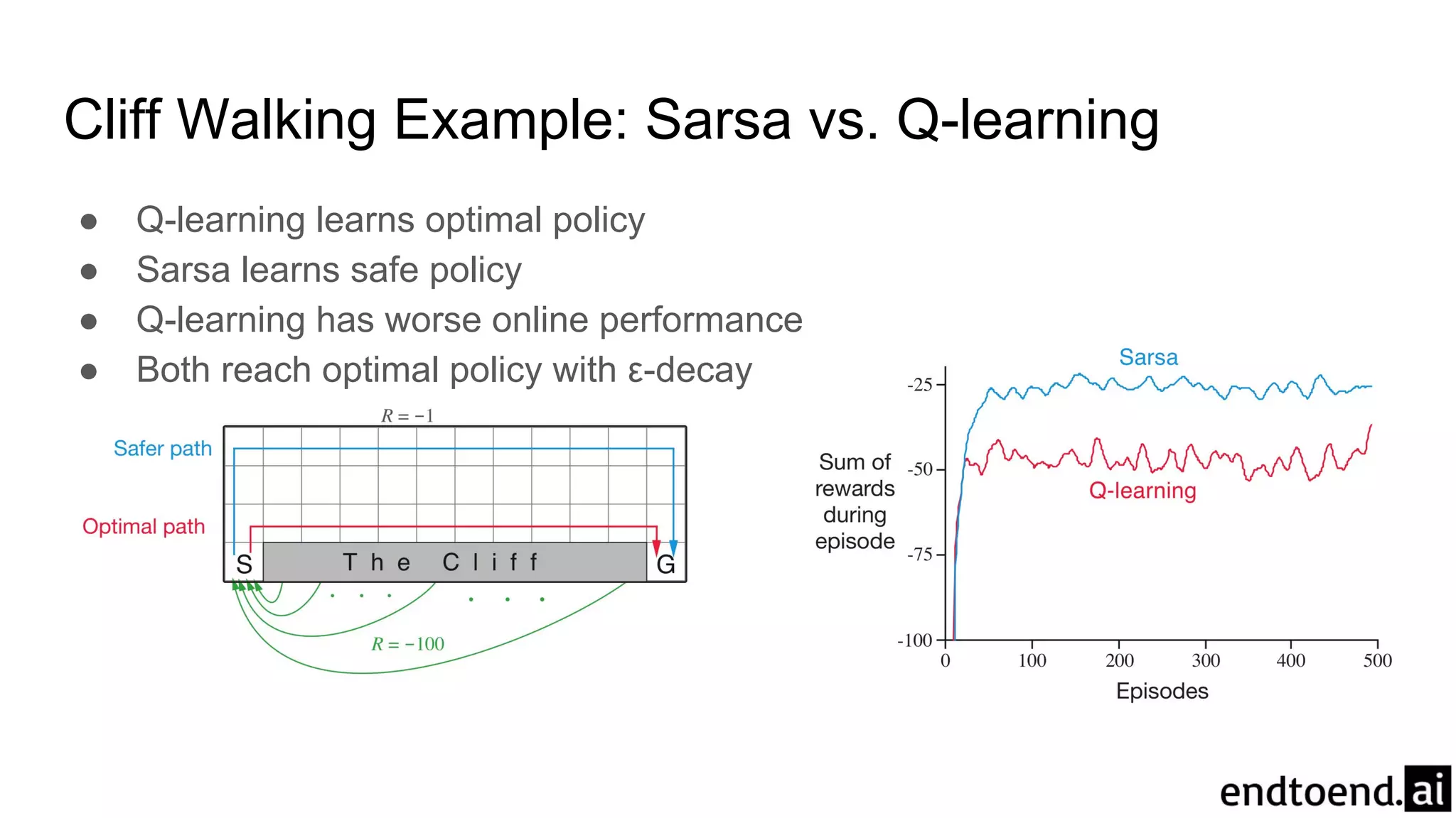
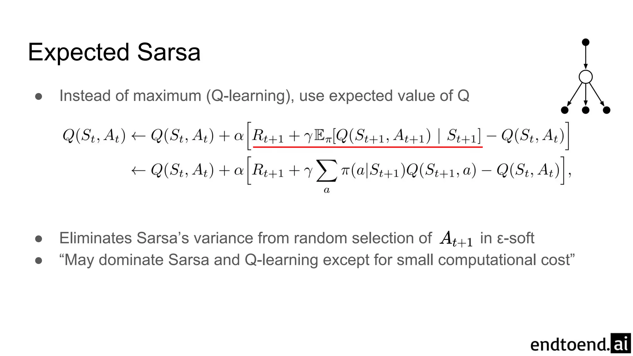
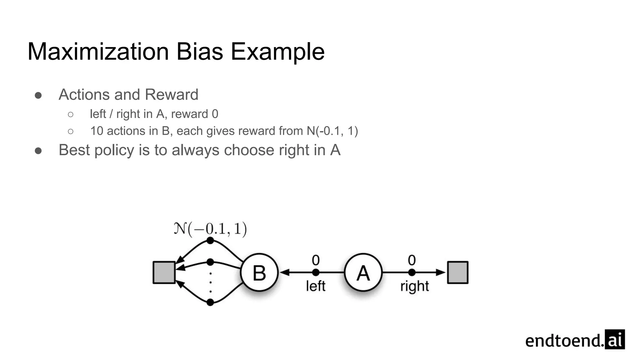
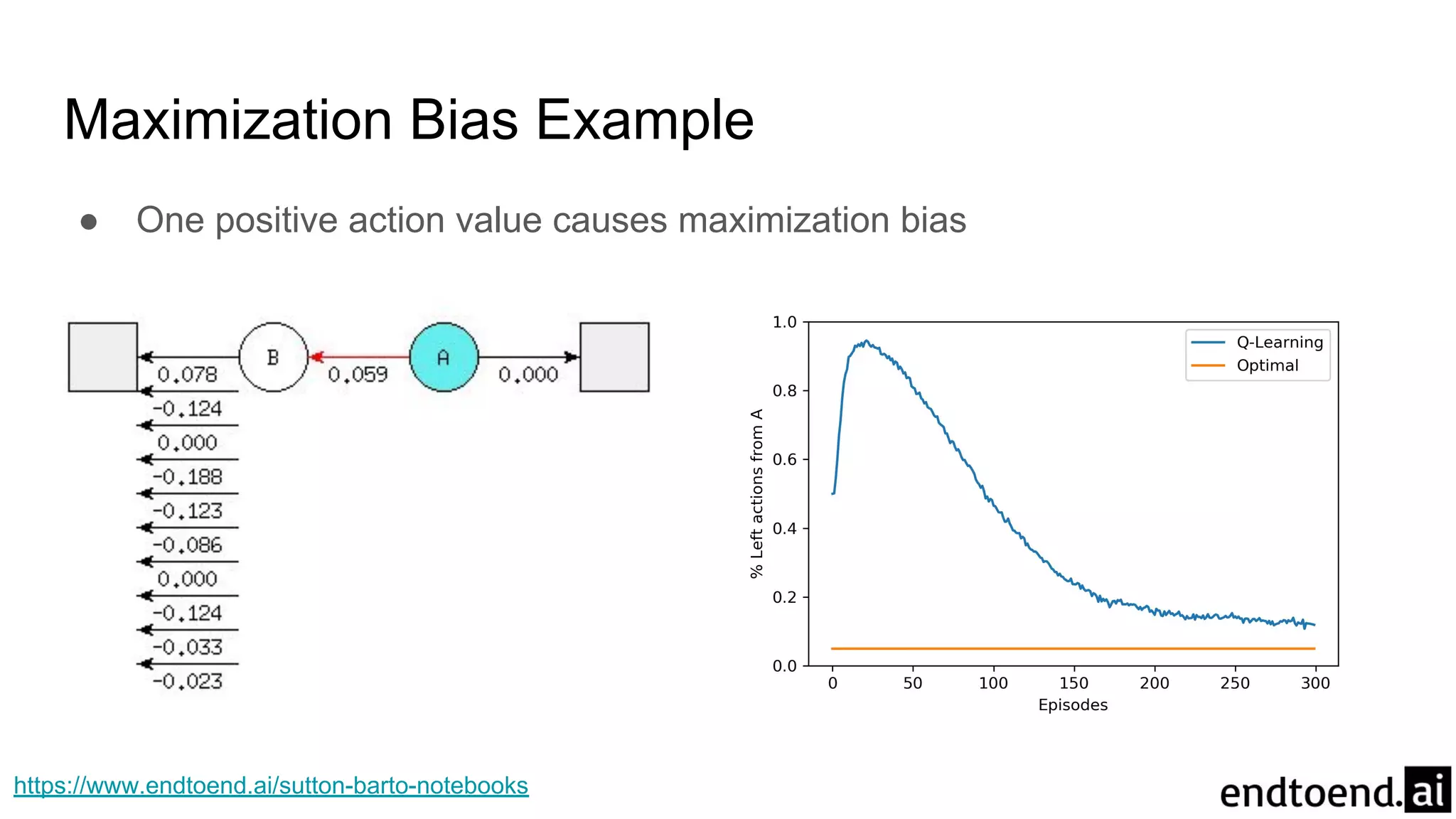
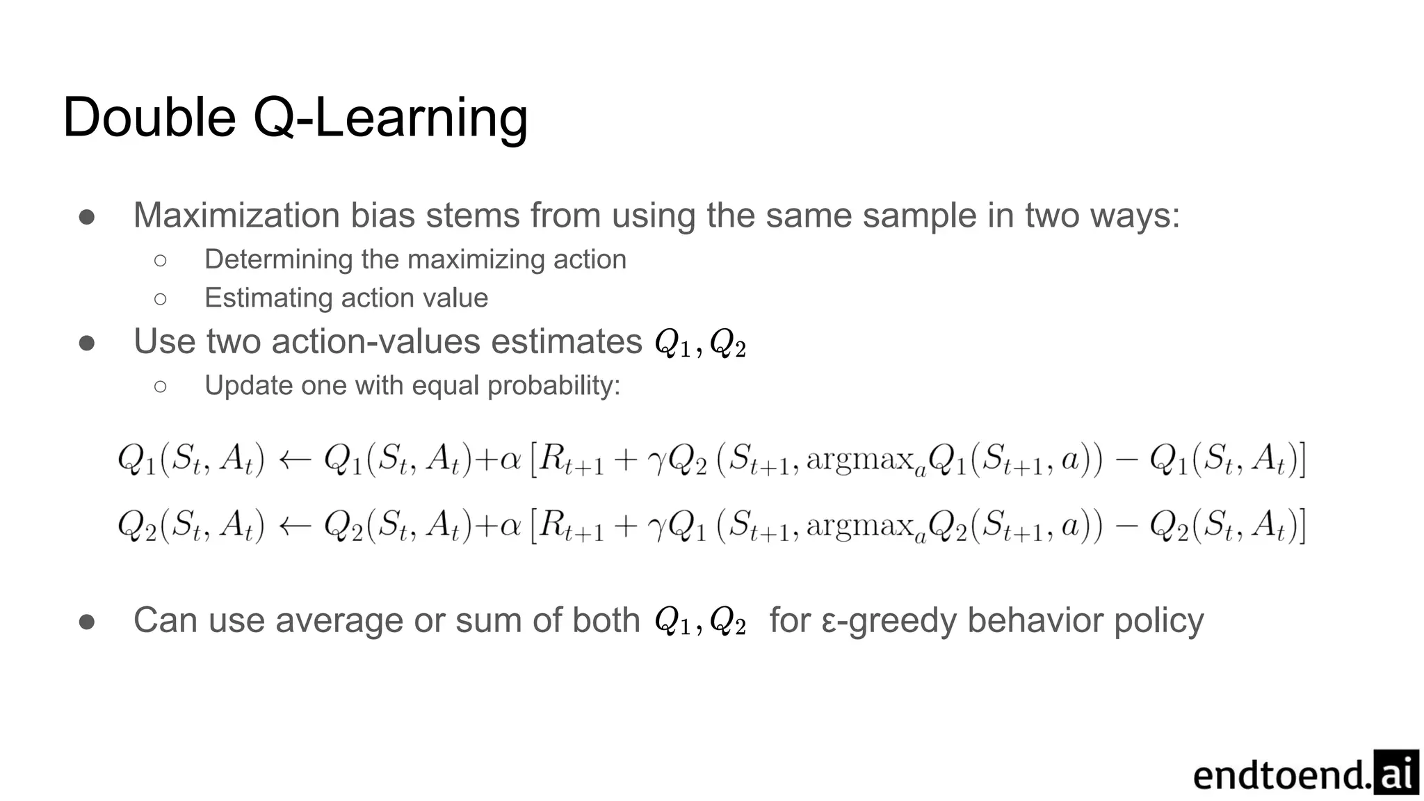
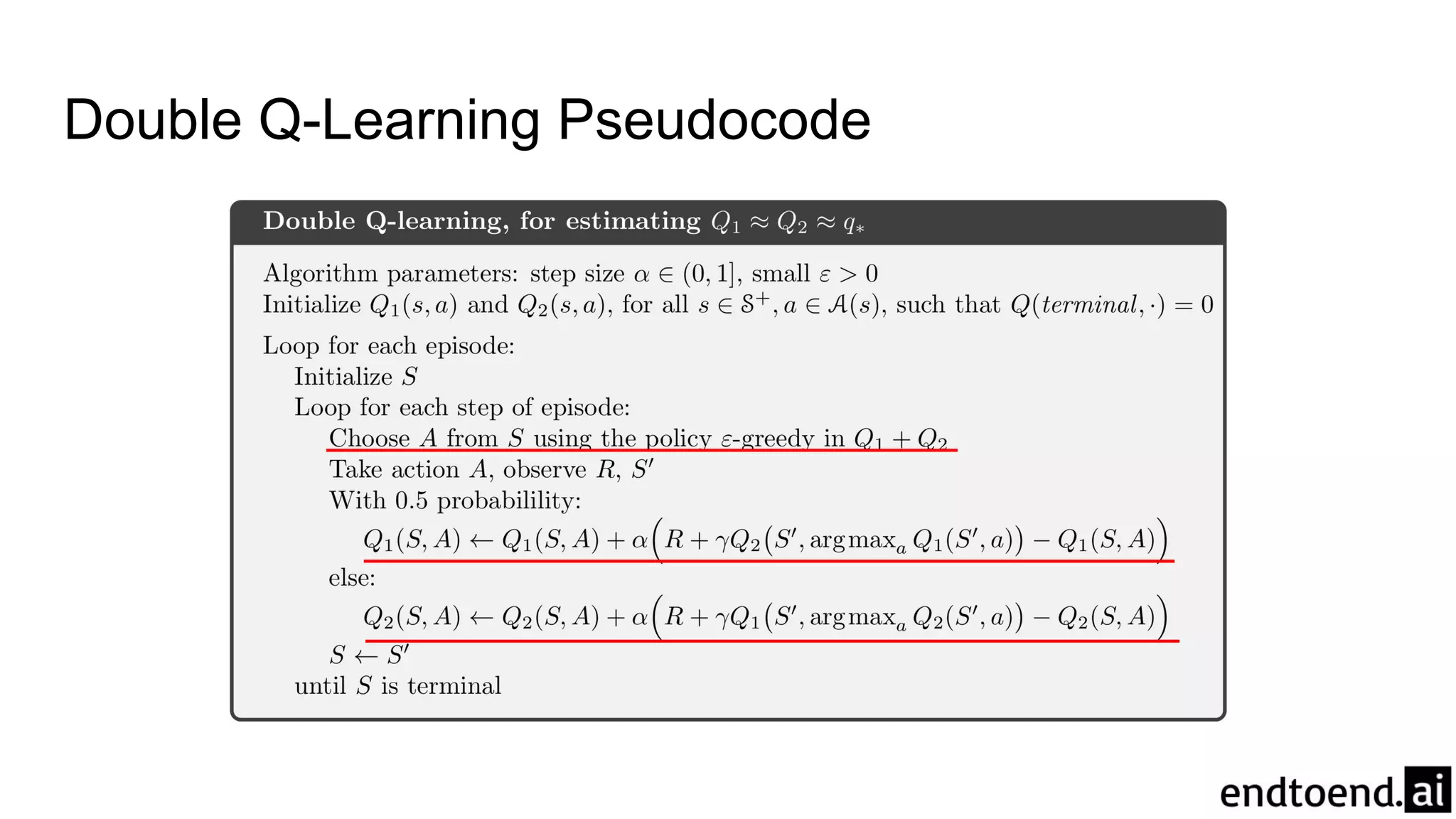
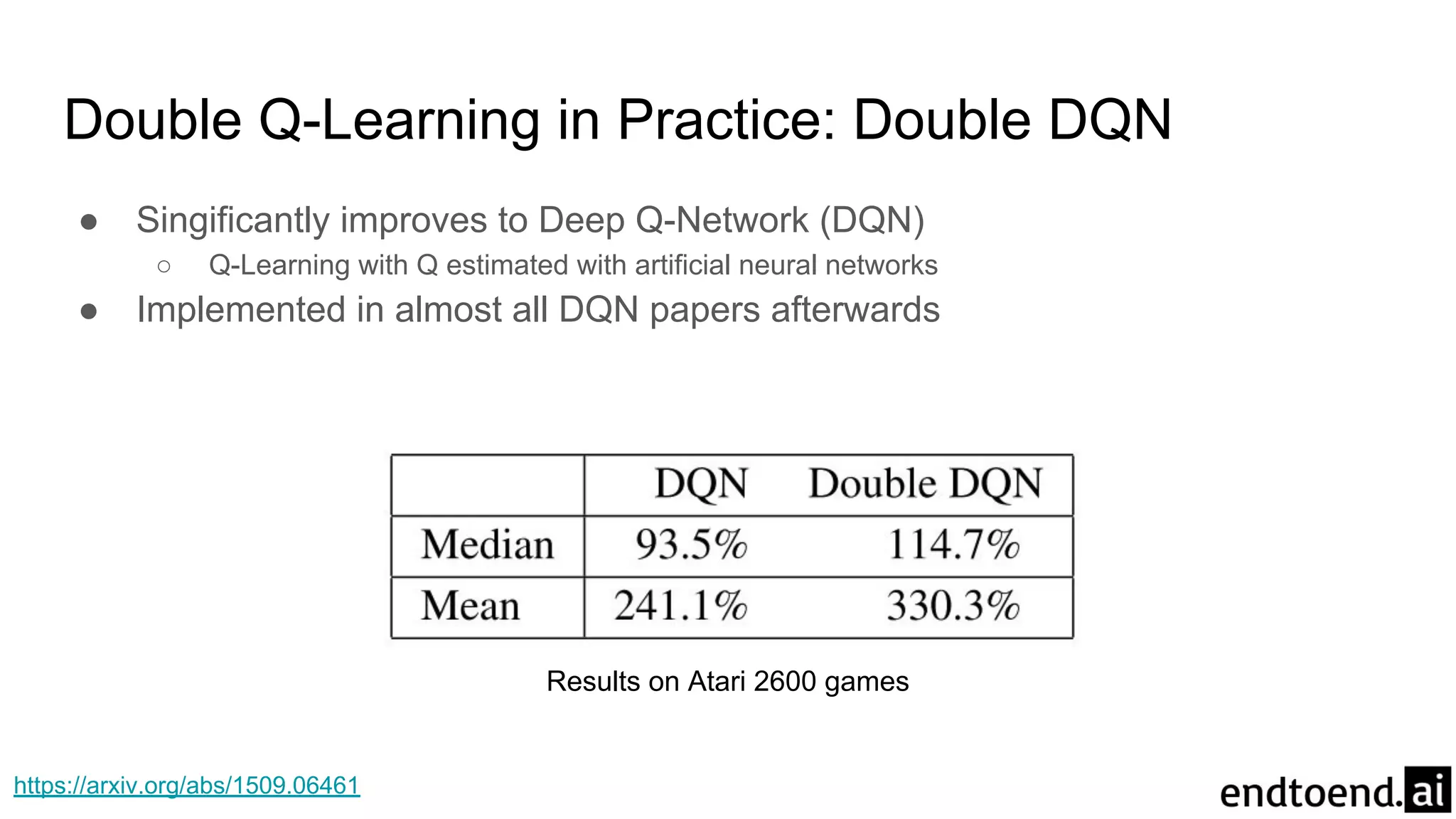
Chapter 6: Temporal-Difference Learning
Seungjae Ryan Lee
Temporal Difference (TD) Learning
● Combine ideas of Dynamic Programming and Monte Carlo
○ Bootstrapping (DP)
○ Learn from experience without model (MC)
DP MC TD
http://www0.cs.ucl.ac.uk/staff/d.silver/web/Teaching_files/MC-TD.pdf
● Monte Carlo: wait until end of episode
● 1-step TD / TD(0): wait until next time step
Bootstrapping target
TD error
MC error
One-step TD Prediction
One-step TD Prediction Pseudocode
Driving Home Example
● Predict how long it takes to drive home
○ Reward: Elapsed time for each segment
○ Value of state: expected time to go
Driving Home Example: MC vs TD
Advantages of TD Prediction methods
● vs. Dynamic Programming
○ No model required
● vs. Monte Carlo
○ Allows online incremental learning
○ Does not need to ignore episodes with experimental actions
● Still guarantees convergence
● Converges faster than MC in practice
○ ex) Random Walk
○ No theoretical results yet
Random Walk Example
● Start at C, move left/right with equal probability
● Only nonzero reward is
● True state values:
● 100 episodes for MC and TD(0)
● All value estimates initialized to 0.5
Random Walk Example: Convergence
● Converges to true value
○ Not exactly due to step size
Random Walk Example: MC vs. TD(0)
● RMS error decreases faster in TD(0)
Batch Updating
Episode 1
Episode 2
Episode 3
Batch 1
Batch 2
Batch 3
● Repeat learning from same experience until convergence
● Useful when finite amount of experience is available
● Convergence guaranteed with small step-size parameter
● MC and TD converge to different answers
ex)
You are the Predictor Example
● Suppose you observe 8 episodes:
● V(B) = 6 / 8
● What is V(A)?
You are the Predictor Example: Batch MC
● State A had zero return in 1 episode → V(A) = 0
● Minimize mean-squared error (MSE) on the training set
○ Zero error on the 8 episodes
○ Does not use the Markov property or sequential property within episode
A
1
B
1 1 1 00 1 1 1
You are the Predictor Example: Batch TD(0)
● A went to B 100% of the time → V(A) = V(B) = 6 / 8
● Create a best-fit model of the Markov process from the training set
○ Model = maximum likelihood estimate (MLE)
● If the model is exactly correct, we can compute the true value function
○ Known as the certainty-equivalence estimate
○ Direct computation is unfeasible ( memory, computations)
● TD(0) converges to the certainty-equivalence estimate
○ memory needed
Random Walk Example: Batch Updating
● Batch TD(0) has consistently lower RMS error than Batch MC
Sarsa: On-policy TD Control
● Learn action-value function with TD(0)
● Use transition for updates
● Change policy greedily with
● Converges if:
○ all is visited infinitely many times
○ policy converges to greedy policy
TD error
Sarsa: On-Policy TD Control Pseudocode
Windy Gridworld Example
● Gridworld with “Wind”
○ Actions: 4 directions
○ Reward: -1 until goal
○ “Wind” at each column shifts agent upward
○ “Wind” strength varies by column
● Termination not guaranteed for all policies
● Monte Carlo cannot be used easily
Windy Gridworld Example
● Converges at 17 steps (instead of optimal 15) due to exploring policy
Q-learning: Off-policy TD Control
● directly approximates independent of behavior policy
● Converges if all is visited infinitely many times
Q-learning: Off-policy TD Control: Pseudocode
Cliff Walking Example
● Gridworld with “cliff” with high negative reward
● ε-greedy (behavior) policy for both Sarsa and Q-learning (ε = 0.1)
Cliff Walking Example: Sarsa vs. Q-learning
● Q-learning learns optimal policy
● Sarsa learns safe policy
● Q-learning has worse online performance
● Both reach optimal policy with ε-decay
Expected Sarsa
● Instead of maximum (Q-learning), use expected value of Q
● Eliminates Sarsa’s variance from random selection of in ε-soft
● “May dominate Sarsa and Q-learning except for small computational cost”
Cliff Walking Example: Parameter Study
Maximization Bias
● All shown control algorithms involve maximization
○ Sarsa: ε-greedy policy
○ Q-learning: greedy target policy
● Can introduce significant positive bias that hinders learning
Maximization Bias Example
● Actions and Reward
○ left / right in A, reward 0
○ 10 actions in B, each gives reward from N(-0.1, 1)
● Best policy is to always choose right in A
Maximization Bias Example
● One positive action value causes maximization bias
https://www.endtoend.ai/sutton-barto-notebooks
Double Q-Learning
● Maximization bias stems from using the same sample in two ways:
○ Determining the maximizing action
○ Estimating action value
● Use two action-values estimates
○ Update one with equal probability:
● Can use average or sum of both for ε-greedy behavior policy
Double Q-Learning Pseudocode
Double Q-Learning Result
Double Q-Learning in Practice: Double DQN
● Singificantly improves to Deep Q-Network (DQN)
○ Q-Learning with Q estimated with artificial neural networks
● Implemented in almost all DQN papers afterwards
Results on Atari 2600 games
https://arxiv.org/abs/1509.06461
Afterstate Value Functions
● Evaluate the state after the action (afterstate)
● Useful when:
○ the immediate effect of action is known
○ multiple can lead to same afterstate
Summary
● Can be applied on-line with minimal amount of computation
● Uses experience generated from interaction
● Expressed simply by single equations
→ Used most widely in Reinforcement Learning
● This was one-step, tabular, model-free TD methods
● Can be extended in all three ways to be more powerful
Thank you!
Original content from
● Reinforcement Learning: An Introduction by Sutton and Barto
You can find more content in
● github.com/seungjaeryanlee
● www.endtoend.ai

Reinforcement Learning 6. Temporal Difference Learning

  • 1.
    Chapter 6: Temporal-DifferenceLearning Seungjae Ryan Lee
  • 2.
    Temporal Difference (TD)Learning ● Combine ideas of Dynamic Programming and Monte Carlo ○ Bootstrapping (DP) ○ Learn from experience without model (MC) DP MC TD http://www0.cs.ucl.ac.uk/staff/d.silver/web/Teaching_files/MC-TD.pdf
  • 3.
    ● Monte Carlo:wait until end of episode ● 1-step TD / TD(0): wait until next time step Bootstrapping target TD error MC error One-step TD Prediction
  • 4.
  • 5.
    Driving Home Example ●Predict how long it takes to drive home ○ Reward: Elapsed time for each segment ○ Value of state: expected time to go
  • 6.
  • 7.
    Advantages of TDPrediction methods ● vs. Dynamic Programming ○ No model required ● vs. Monte Carlo ○ Allows online incremental learning ○ Does not need to ignore episodes with experimental actions ● Still guarantees convergence ● Converges faster than MC in practice ○ ex) Random Walk ○ No theoretical results yet
  • 8.
    Random Walk Example ●Start at C, move left/right with equal probability ● Only nonzero reward is ● True state values: ● 100 episodes for MC and TD(0) ● All value estimates initialized to 0.5
  • 9.
    Random Walk Example:Convergence ● Converges to true value ○ Not exactly due to step size
  • 10.
    Random Walk Example:MC vs. TD(0) ● RMS error decreases faster in TD(0)
  • 11.
    Batch Updating Episode 1 Episode2 Episode 3 Batch 1 Batch 2 Batch 3 ● Repeat learning from same experience until convergence ● Useful when finite amount of experience is available ● Convergence guaranteed with small step-size parameter ● MC and TD converge to different answers ex)
  • 12.
    You are thePredictor Example ● Suppose you observe 8 episodes: ● V(B) = 6 / 8 ● What is V(A)?
  • 13.
    You are thePredictor Example: Batch MC ● State A had zero return in 1 episode → V(A) = 0 ● Minimize mean-squared error (MSE) on the training set ○ Zero error on the 8 episodes ○ Does not use the Markov property or sequential property within episode A 1 B 1 1 1 00 1 1 1
  • 14.
    You are thePredictor Example: Batch TD(0) ● A went to B 100% of the time → V(A) = V(B) = 6 / 8 ● Create a best-fit model of the Markov process from the training set ○ Model = maximum likelihood estimate (MLE) ● If the model is exactly correct, we can compute the true value function ○ Known as the certainty-equivalence estimate ○ Direct computation is unfeasible ( memory, computations) ● TD(0) converges to the certainty-equivalence estimate ○ memory needed
  • 15.
    Random Walk Example:Batch Updating ● Batch TD(0) has consistently lower RMS error than Batch MC
  • 16.
    Sarsa: On-policy TDControl ● Learn action-value function with TD(0) ● Use transition for updates ● Change policy greedily with ● Converges if: ○ all is visited infinitely many times ○ policy converges to greedy policy TD error
  • 17.
    Sarsa: On-Policy TDControl Pseudocode
  • 18.
    Windy Gridworld Example ●Gridworld with “Wind” ○ Actions: 4 directions ○ Reward: -1 until goal ○ “Wind” at each column shifts agent upward ○ “Wind” strength varies by column ● Termination not guaranteed for all policies ● Monte Carlo cannot be used easily
  • 19.
    Windy Gridworld Example ●Converges at 17 steps (instead of optimal 15) due to exploring policy
  • 20.
    Q-learning: Off-policy TDControl ● directly approximates independent of behavior policy ● Converges if all is visited infinitely many times
  • 21.
    Q-learning: Off-policy TDControl: Pseudocode
  • 22.
    Cliff Walking Example ●Gridworld with “cliff” with high negative reward ● ε-greedy (behavior) policy for both Sarsa and Q-learning (ε = 0.1)
  • 23.
    Cliff Walking Example:Sarsa vs. Q-learning ● Q-learning learns optimal policy ● Sarsa learns safe policy ● Q-learning has worse online performance ● Both reach optimal policy with ε-decay
  • 24.
    Expected Sarsa ● Insteadof maximum (Q-learning), use expected value of Q ● Eliminates Sarsa’s variance from random selection of in ε-soft ● “May dominate Sarsa and Q-learning except for small computational cost”
  • 25.
    Cliff Walking Example:Parameter Study
  • 26.
    Maximization Bias ● Allshown control algorithms involve maximization ○ Sarsa: ε-greedy policy ○ Q-learning: greedy target policy ● Can introduce significant positive bias that hinders learning
  • 27.
    Maximization Bias Example ●Actions and Reward ○ left / right in A, reward 0 ○ 10 actions in B, each gives reward from N(-0.1, 1) ● Best policy is to always choose right in A
  • 28.
    Maximization Bias Example ●One positive action value causes maximization bias https://www.endtoend.ai/sutton-barto-notebooks
  • 29.
    Double Q-Learning ● Maximizationbias stems from using the same sample in two ways: ○ Determining the maximizing action ○ Estimating action value ● Use two action-values estimates ○ Update one with equal probability: ● Can use average or sum of both for ε-greedy behavior policy
  • 30.
  • 31.
  • 32.
    Double Q-Learning inPractice: Double DQN ● Singificantly improves to Deep Q-Network (DQN) ○ Q-Learning with Q estimated with artificial neural networks ● Implemented in almost all DQN papers afterwards Results on Atari 2600 games https://arxiv.org/abs/1509.06461
  • 33.
    Afterstate Value Functions ●Evaluate the state after the action (afterstate) ● Useful when: ○ the immediate effect of action is known ○ multiple can lead to same afterstate
  • 34.
    Summary ● Can beapplied on-line with minimal amount of computation ● Uses experience generated from interaction ● Expressed simply by single equations → Used most widely in Reinforcement Learning ● This was one-step, tabular, model-free TD methods ● Can be extended in all three ways to be more powerful
  • 35.
    Thank you! Original contentfrom ● Reinforcement Learning: An Introduction by Sutton and Barto You can find more content in ● github.com/seungjaeryanlee ● www.endtoend.ai