Download as PDF, PPTX
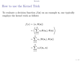
![Kernels
Some Definitions
Definition 1.1 (Positive Definite Kernel)
Let X be a nonempty set. A function k : X × X → C is called a
positive definite if and only if
n∑
i=1
n∑
j=1
cicjk(xi, xj) ≥ 0 (1)
for all n ∈ N, {x1, . . . , xn} ⊆ X and {c1, . . . , cn}.
Unfortunately, there is no common use of the preceding definition in
the literature. Indeed, some authors call positive definite function
positive semi-definite, ans strictly positive definite functions are
sometimes called positive definite.
Note:
For fixed x1, x2, . . . , xn ∈ X, then n × n matrix K := [k(xi, xj)]1≤i,j≤n
is often called the Gram Matrix.
6 / 28](https://image.slidesharecdn.com/second-lecture-150902220946-lva1-app6891/85/Kernels-and-Support-Vector-Machines-6-320.jpg)
![Kernels
Mercer Condition
Theorem 1.2
Let X = [a, b] be compact interval and let k : [a, b] × [a, b] → C be
continuous. Then φ is positive definite if and only if
∫ b
a
∫ b
a
c(x)c(y)k(x, y)dxdy ≥ 0 (2)
for each continuous function c : X → C.
7 / 28](https://image.slidesharecdn.com/second-lecture-150902220946-lva1-app6891/85/Kernels-and-Support-Vector-Machines-7-320.jpg)


![Kernels Kernel Families
References for Kernels
[3] C. Berg, J. Reus, and P. Ressel. Harmonic Analysis on
Semigroups: Theory of Positive Definite and Related Functions.
Springer Science+Business Media, LLV, 1984.
[9] Felipe Cucker and Ding Xuan Zhou. Learning Theory.
Cambridge University Press, 2007.
[47] Ingo Steinwart and Christmannm Andreas. Support Vector
Machines. 2008.
16 / 28](https://image.slidesharecdn.com/second-lecture-150902220946-lva1-app6891/85/Kernels-and-Support-Vector-Machines-16-320.jpg)
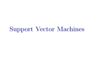

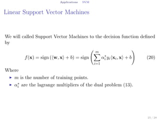
![Applications SVM
Proof.
The Lagrangianx of the function F is
L(x, b, α) =
1
2
∥w∥2
−
m∑
i=1
αi[yi(⟨w, xi⟩ + b) − 1] (12)
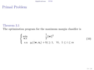
Because of the KKT conditions are hold (F is continuous and
differentiable and the restrictions are also continuous and differentiable)
then we can add the complementary conditions
Stationarity:
∇wL = w −
m∑
i=1
αiyixi = 0 ⇒ w =
m∑
i=1
αiyixi (13)
∇bL = −
m∑
i=1
αiyi = 0 ⇒
m∑
i=1
αiyi = 0 (14)
22 / 28](https://image.slidesharecdn.com/second-lecture-150902220946-lva1-app6891/85/Kernels-and-Support-Vector-Machines-22-320.jpg)
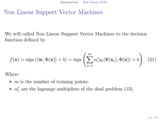
![Applications SVM
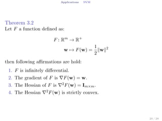
Primal feasibility:
yi(⟨w, xi⟩ + b) ≥ 1, ∀i ∈ [1, m] (15)
Dual feasibility:
αi ≥ 0, ∀i ∈ [1, m] (16)
Complementary slackness:
αi[yi(⟨w, xi⟩+b)−1] = 0 ⇒ αi = 0∨yi(⟨w, xi⟩+b) = 1, ∀i ∈ [1, m] (17)
L(w, b, α) =
1
2
m∑
i=1
αiyixi
2
−
m∑
i=1
m∑
j=1
αiαjyiyj⟨xi, xj⟩
=− 1
2
∑m
i=1
∑m
j=1 αiαjyiyj⟨xi,xj⟩
−
m∑
i=1
αiyib
=0
+
m∑
i=1
αi
(18)
then
L(w, b, α) =
m∑
i=1
αi −
1
2
m∑
i=1
m∑
j=1
αiαjyiyj⟨xi, xj⟩ (19)
23 / 28](https://image.slidesharecdn.com/second-lecture-150902220946-lva1-app6891/85/Kernels-and-Support-Vector-Machines-23-320.jpg)
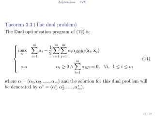
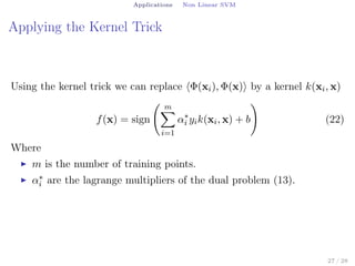
![Applications SVM
Theorem 3.4
Let G a function defined as:
G: Rm
→ R
α → G(α) = αt
Im×m −
1
2
αt
Aα
where α = (α1, α2, . . . , αm) y A = [yiyj⟨xi, xj⟩]1≤i,j≤m in Rm×m then
the following affirmations are hold:
1. The A is symmetric.
2. The function G is differentiable and
∂G(α)
∂α
= Im×m − Aα.
3. The function G is twice differentiable and
∂2G(α)
∂α2
= −A.
4. The function G is a concave function.
24 / 28](https://image.slidesharecdn.com/second-lecture-150902220946-lva1-app6891/85/Kernels-and-Support-Vector-Machines-24-320.jpg)
![Applications Non Linear SVM
References for Support Vector Machines
[31] Mehryar Mohri, Afshin Rostamizadeh, and Ameet Talwalkar.
Foundations of Machine Learning. The MIT Press, 2012.
28 / 28](https://image.slidesharecdn.com/second-lecture-150902220946-lva1-app6891/85/Kernels-and-Support-Vector-Machines-28-320.jpg)

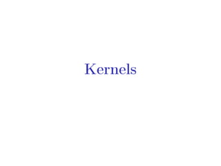
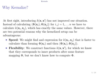
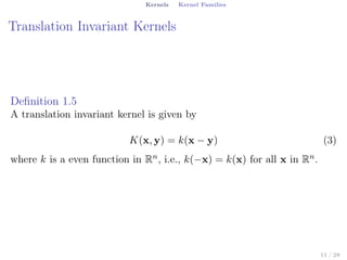
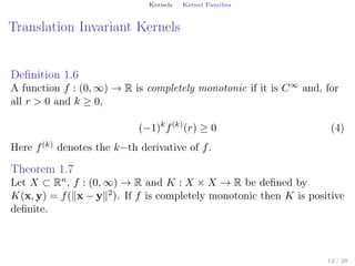
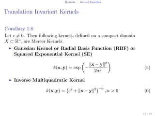
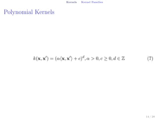
This document summarizes a seminar on kernels and support vector machines. It begins by explaining why kernels are useful for increasing flexibility and speed compared to direct inner product calculations. It then covers definitions of positive definite kernels and how to prove a function is a kernel. Several kernel families are discussed, including translation invariant, polynomial, and non-Mercer kernels. Finally, the document derives the primal and dual problems for support vector machines and explains how the kernel trick allows non-linear classification.


![Polymer [ बहुलक ] Chemistry Notes PDF - Irfanullah Mehar - JJ Sir Chemistry.pdf](https://cdn.slidesharecdn.com/ss_thumbnails/polymerchemistrynotespdf-irfanullahmehar-jjsirchemistry-260210172118-3f9b37f7-thumbnail.jpg?width=640&height=640&fit=bounds)


