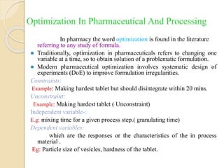
OPTIMIZATION TECHNIQUES Optimization techniques are methods for achieving the best possible result under given constraints. There are various classical and advanced optimization methods. Classical methods include techniques for single-variable, multi-variable without constraints, and multi-variable with equality or inequality constraints using methods like Lagrange multipliers or Kuhn-Tucker conditions. Advanced methods include hill climbing, simulated annealing, genetic algorithms, and ant colony optimization. Optimization has applications in fields like engineering, business/economics, and pharmaceutical formulation to improve processes and outcomes under constraints.

1. OPTIMIZATION
TECHNIQUES

2. Definition:
 An optimization is the act of achieving the
best possible result under given
circumstances.
 Primary objective may not be optimize
absolutely but to compromise effectively
&thereby produce the best formulation under a
given set of restrictions .

3. 3
optimization
Reduce
the cost
Safety &
reduce the
error
reproducibilit
y
Save the
time
Why Optimization is necessary?
Innovation
&
efficiency

4. Historical development
 Isaac Newton (1642-1727) :The development of differential
calculus methods of optimization.
 Joseph-Louis Lagrange (1736-1813) :Calculus of variations,
minimization of functionals, method of optimization for
constrained problems.
 Augustin-Louis Cauchy (1789-1857) :Solution by direct
substitution, steepest descent method for unconstrained
optimization.
 George Bernard Dantzig (1914-2005):Linear programming
and Simplex method (1947).
 Albert William Tucker (1905-1995):Necessary and sufficient
conditions for the optimal solution of programming problems,
nonlinear programming.

5. OPTIMIZATION PARAMETERS
 Objective function
An objective function expresses the main aim
of the model which is either to be minimized or
maximized.
 For example: in a manufacturing process, the aim may be
to maximize the profit or minimize the cost.
 The two exceptions are:
• No objective function
• Multiple objective functions.

6. Variables
A set of unknowns or variables control the value of
the objective function.
variables can be broadly classified as:
• Independent variable
• Dependent variable
Constraints
The restrictions that must be satisfied to produce an
acceptable design are collectively called design constraints.
Constraints can be broadly classified as:
•Behavioral or Functional
•Geometric or Side

7. Statement of an optimization problem
 An optimization problem can be stated as follows:
To find X =
which minimizes f(X)
Subject to the constraints
gi(X) ≤ 0 , i = 1, 2, …., m
lj(X) = 0, j = 1, 2, …., p
where X is an n-dimensional vector called the design vector,
f(X) is called the objective function, and gi(X) and lj(X) are
known as inequality and equality constraints, respectively.

8. Classification of optimization
 Based on Constraints
◦ Constrained optimization (Lagrangian method)
◦ Unconstrained optimization (Least Squares)
 Based on Nature of the design variables
◦ Static optimization
◦ Dynamic optimization
 Based on Physical structure
◦ Optimal control
◦ Sub-optimal control

9. •Based on Nature of variables
• Stochastic optimization
• Deterministic optimization
• Based On Separability Of The Functions
• Separable
•Non separable
Based on the Nature of the Equations Involved
• Linear programming
• Quadratic programming
• Nonlinear programming

10. Based on the Permissible Values of the Design Variables
•Inter programming
•Real valued programming
Based on the Number of Objective Functions
•Single objective
•Multi objective

11. Classical Optimization
 The classical methods of optimization are useful in
finding the optimum solution of continuous and
differentiable functions.
classical optimization techniques, can handle 3 types of
problems:
i. single variable functions
ii. multivariable functions with no constraints
iii. multivariable functions with both equality and
inequality constraints

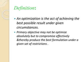
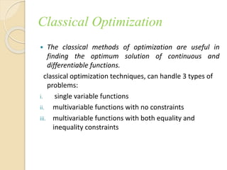
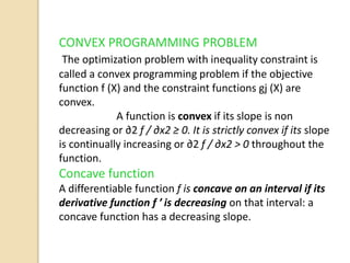
12. Single variable optimization:
 A single-variable optimization problem is one in which
the value of x = x ∗ is to be found in the interval [a, b]
such that x ∗ minimizes f (x).
f (x) at x = x ∗ is said to have a
local minimum if f (x∗ ) ≤ f (x∗ + h) for all small ± h
local maximum if f (x∗ ) ≥ f (x∗ + h) for all values of
h≈0
Global minimum if f (x∗ ) ≤ f (x) for all x
Global maximum if f (x∗ ) ≥ f (x) for all x

13. MULTIVARIABLE OPTIMIZATION WITH NO CONSTRAINTS
 It is the minimum or maximum of an unconstrained
function of several variables
Necessary Condition
If f (X) has an extreme point (max or min) at X = X ∗ and if
the first partial derivatives of f (X) exist at X ∗ , then
∂f /∂x1 (X ∗ ) = ∂f/ ∂x2 (X ∗ ) = · · · = ∂f /∂xn (X ∗ ) = 0
Sufficient Condition
The Hessian matrix defined by H is made using the second
order derivatives
(i) positive definite when X ∗ is a relative minimum
point
(ii) negative definite when X ∗ is a relative maximum
point.

14. MULTIVARIABLE WITH EQUALITY CONSTRAINTS
Minimize f= f(X)
Subject to the constraints
gi(X) =0 , i = 1, 2, …., m
where X=
 Here m ≤n; otherwise (if m > n), the problem becomes
over defined and, in general, there will be no solution.
 There are several methods available for the solution of
this problem
Such methods are
1. Direct substitution
2 .Constrained variation
3. Lagrange multipliers

15. Solution by Direct Substitution
 A problem with n variables and m equality constraints, ,
it is theoretically possible to solve simultaneously the m
equality constraints and express any set of m variables
in terms of the remaining n − m variables.
 With these new objective unction is obtained.
Drawbacks
 constraint equations will be nonlinear for most of
practical problems.
 often it becomes impossible to solve them and express
any m variables in terms of the remaining n − m
variables.

16. By the Method of Constrained Variation
 The basic idea used in the method of constrained
variation is to find a closed-form expression for
the first-order differential of f (df) at all points at
which the constraints gj (X) = 0, j = 1, 2, . . . , m,
are satisfied.
Drawback
Prohibitive for problems with more
than three constraints.

17. By The Method Of Lagrange Multipliers
For instance consider the optimization problem
maximize f(x1, x2)
subject to g(x1, x2) = c.
We introduce a new variable (λ) called a Lagrange
multiplier and Lagrange function is defined by
L(x1, x2, λ) = f (x1, x2) + λg(x1, x2)
By treating L as a function of the three variables
x1, x2, and λ, the necessary conditions for its
extreme are given by
∂L/∂x1(x1, x2, λ)= ∂f /∂x1(x1, x2)+ λ ∂g /∂x1(x1, x2) = 0
∂L/∂x2 (x1, x2, λ) = ∂f /∂x2 (x1, x2) + λ ∂g/ ∂x2 (x1, x2) = 0
∂L/ ∂λ (x1, x2, λ) = g(x1, x2) = 0

18. MULTIVARIABLE OPTIMIZATION WITH INEQUALITY
CONSTRAINTS
 The inequality constraints can be transformed to
equality constraints by adding nonnegative slack
variables, y ^2 (j ), as
gj (X) + y ^2 (j ) = 0, j = 1, 2, . . . , m
 where the values of the slack variables are yet
unknown. The problem now becomes
Gj (X, Y) = gj (X) + y ^2 (j ) = 0, j = 1, 2, . . . , m
where Y = {y1, y2, . . . , ym} T is the vector of slack
variables
 This problem can be solved conveniently by the method
of Lagrange multipliers.

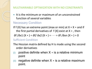
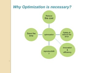
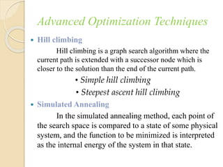
19. Kuhn-Tucker conditions
 Consider the following optimization problem:
Minimize f(X)
subject to gj(X) ≤ 0 for j = 1,2,…,p ;
where X = [x1 x2 . . . xn]
Then the Kuhn-Tucker conditions for X* = [x1 * x2 * . . . xn * ]
to be a local minimum are
∂f /∂xi + ∂gj/∂xi = 0, i = 1, 2, . . . , n
λjgj = 0, j = 1, 2, . . . , m
gj ≤ 0, j = 1, 2, . . . , m
λj ≥ 0, j = 1, 2, . . . , m

20. CONVEX PROGRAMMING PROBLEM
The optimization problem with inequality constraint is
called a convex programming problem if the objective
function f (X) and the constraint functions gj (X) are
convex.
A function is convex if its slope is non
decreasing or ∂2 f / ∂x2 ≥ 0. It is strictly convex if its slope
is continually increasing or ∂2 f / ∂x2 > 0 throughout the
function.
Concave function
A differentiable function f is concave on an interval if its
derivative function f ′ is decreasing on that interval: a
concave function has a decreasing slope.

21. Advanced Optimization Techniques
 Hill climbing
Hill climbing is a graph search algorithm where the
current path is extended with a successor node which is
closer to the solution than the end of the current path.
• Simple hill climbing
• Steepest ascent hill climbing
 Simulated Annealing
In the simulated annealing method, each point of
the search space is compared to a state of some physical
system, and the function to be minimized is interpreted
as the internal energy of the system in that state.

22. Genetic Algorithm:
GAs belong to a class of methods called Evolutionary Algorithms
(EA) that are inspired by the processes of natural selection.
•GAs are different from more traditional optimization techniques because
they search from a population of points rather than a single point.
•They also use payoff information based on an objective function defined
by the user rather than derivatives or other secondary knowledge.
Ant Colony Optimization:
An ACO algorithm is an artificial intelligence technique based on
the pheromone-laying behavior of ants; it can be used to find solutions to
exceedingly complex problems that seek the optimal path through a
graph.
•Ant colony optimization algorithms have been used to produce near-
optimal solutions to the traveling salesman problem.
•The ant colony algorithm can be run continuously and can adapt to

23. Optimization In Managerial
Economics
 The objective of business firm is to maximize
profits or the value of firm or to maximize cost ,
subject to some constraints.
The value of firm is impacted by
• Total Revenue
• Total Cost
Basic economic relations
•Functional Relations
•Total, Average & Marginal Relations
•Graphing Total, Average & Marginal Relations

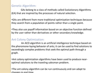
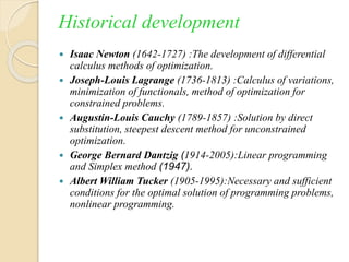
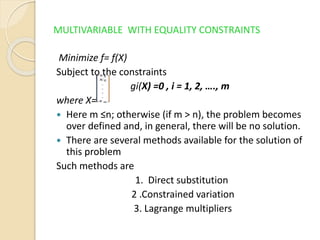
24. Often we wish to optimize but are faced with a constraint. In
such case we need lagrangian multiplier.
L=f(X,Z)+λ[Y-g(X,Z)]
To find the optimal values of x & z, we take derivative of
lagrangian w.r.t X,Z & λ: setting these derivatives to zero.
Example:
A firm faces following cost function
cost=c=f(x,z)=
The firm will produce 80 units of x & z, with any
mix of x & z being acceptable

25. Optimization In Pharmaceutical And Processing
In pharmacy the word optimization is found in the literature
referring to any study of formula.
 Traditionally, optimization in pharmaceuticals refers to changing one
variable at a time, so to obtain solution of a problematic formulation.
 Modern pharmaceutical optimization involves systematic design of
experiments (DoE) to improve formulation irregularities.
Constraints:
Example: Making hardest tablet but should disintegrate within 20 mins.
Unconstraint:
Example: Making hardest tablet ( Unconstraint)
Independent variable-:
E.g: mixing time for a given process step.( granulating time)
Dependent variables:
which are the responses or the characteristics of the in process
material .
Eg: Particle size of vesicles, hardness of the tablet.

26. Statistical Design
Divided into two classes:
•Experimentation continues as the optimization study
proceeds.
Ex: EVOP and simplex methods.
•Experimentation is completed before optimization takes
place.
Ex: Lagrangian method and search methods.
The relationship between dependent and independent
variables can be estimated by two approaches
Theoretical approach.
Empirical or experimental approach.

27. Applications
•To study pharmacokinetic parameters.
•To study process variables in tablet coating operations.
• In high performance liquid chromatography.
•Formulation of culture medium in virology labs.
•Sub micro emulsions with sunscreens using simplex
composite designs.

28. Engineering applications of optimization
 Design of civil engineering structures such as
frames, foundations, bridges, towers, chimneys and
dams for minimum cost.
 Design of minimum weight structures for earth
quake, wind and other types of random loading.
 Shortest route taken by a salesperson visiting
various cities during one tour
 Optimum design of electrical networks
 Optimal plastic design of frame structures
 Design of aircraft and aerospace structure for
minimum weight
 Finding the optimal trajectories of space vehicles.

29. Trajectory Optimization
Minimizing the cost of a space mission is a major concern
in the space industry.
Trajectory optimization has been developed through
classical methods of optimization. However, the
application of Genetic Algorithms has become
increasingly popular.
Objective:
The objective of this optimization was to reduce the time
of-flight and, as a result, the propellant cost.
The Genetic Algorithm used will be responsible for
determining the optimal thrust direction or flight
path angle at the beginning of each time segment
and time-of-flight

30. CONSTRAINTS:
Objective is to minimize the TOF and the penalties to this
minimization are on the position and velocity of the spacecraft at mars
and at Jupiter.
By minimizing the time of flight the risk of damage to the satellite during
the course of the mission is reduced as well as the cost of fuel.

31. SOLUTION OF OPTIMIZATION PROBLEMS USING
MATLAB
 MATLAB is a popular software that is used for
the solution of a variety of scientific and
engineering problems.
 The specific toolbox of interest for solving
optimization and related problems is called the
optimization toolbox.
 Basically, the solution procedure involves three
steps after formulating the optimization
problem

32. step 1
Involves writing an m-file for the objective function.
Step 2
Involves writing an m-file for the constraints.
Step 3
Involves setting the various parameters at proper
values depending on the characteristics of the problem and
the desired output and creating an appropriate file to invoke
the desired MATLAB program.