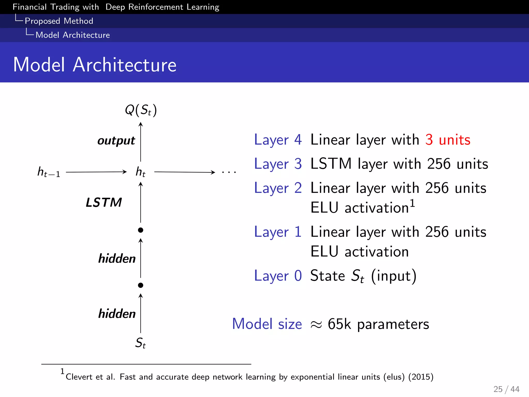
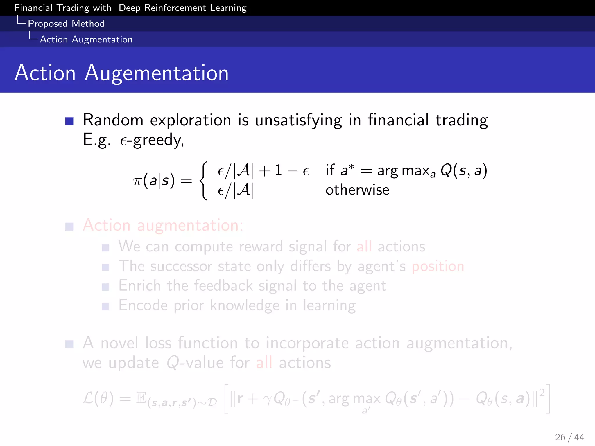
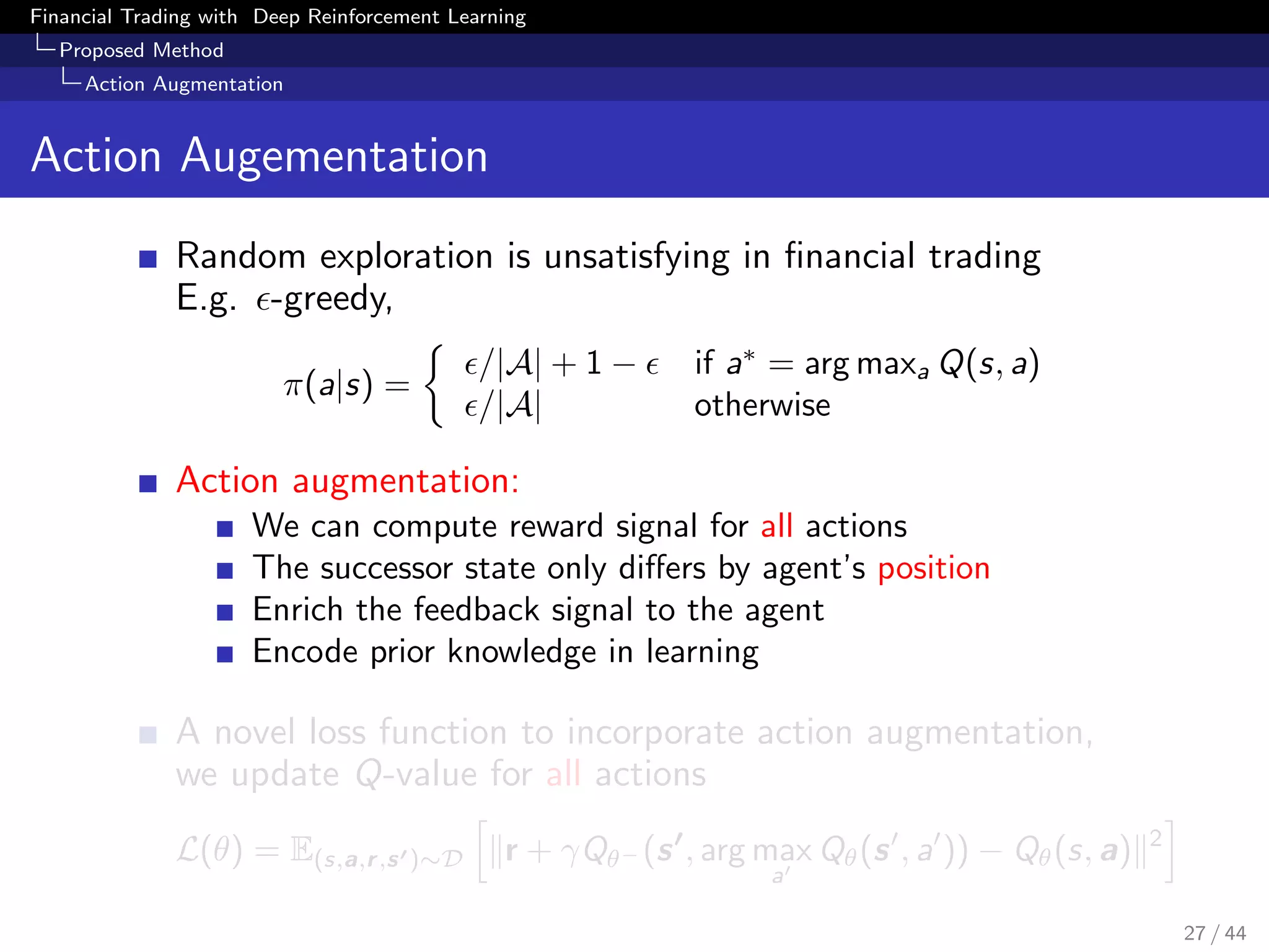
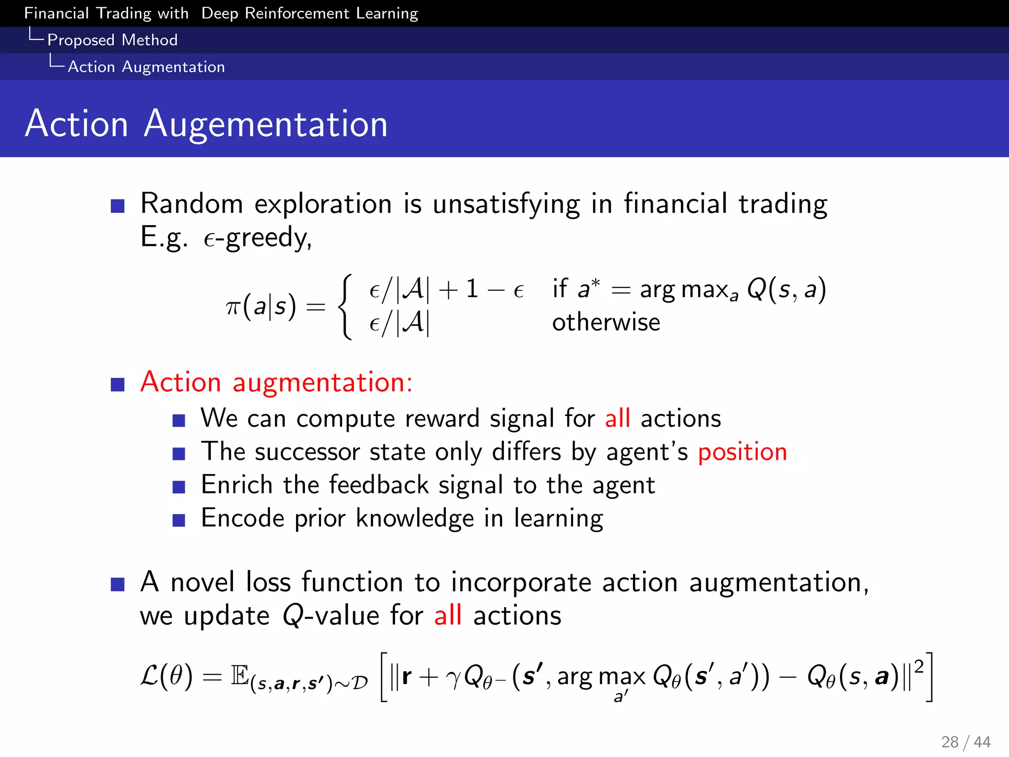
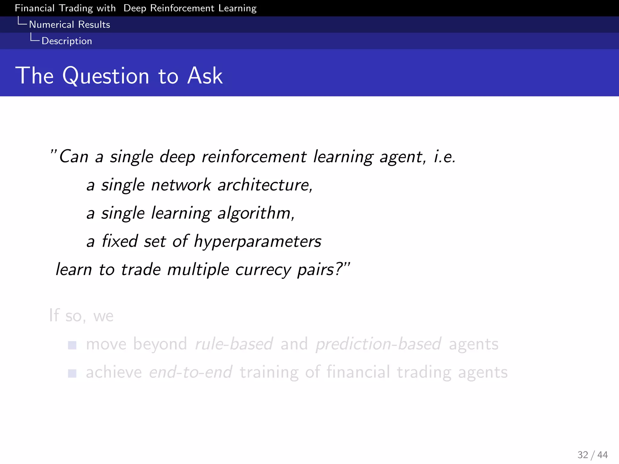
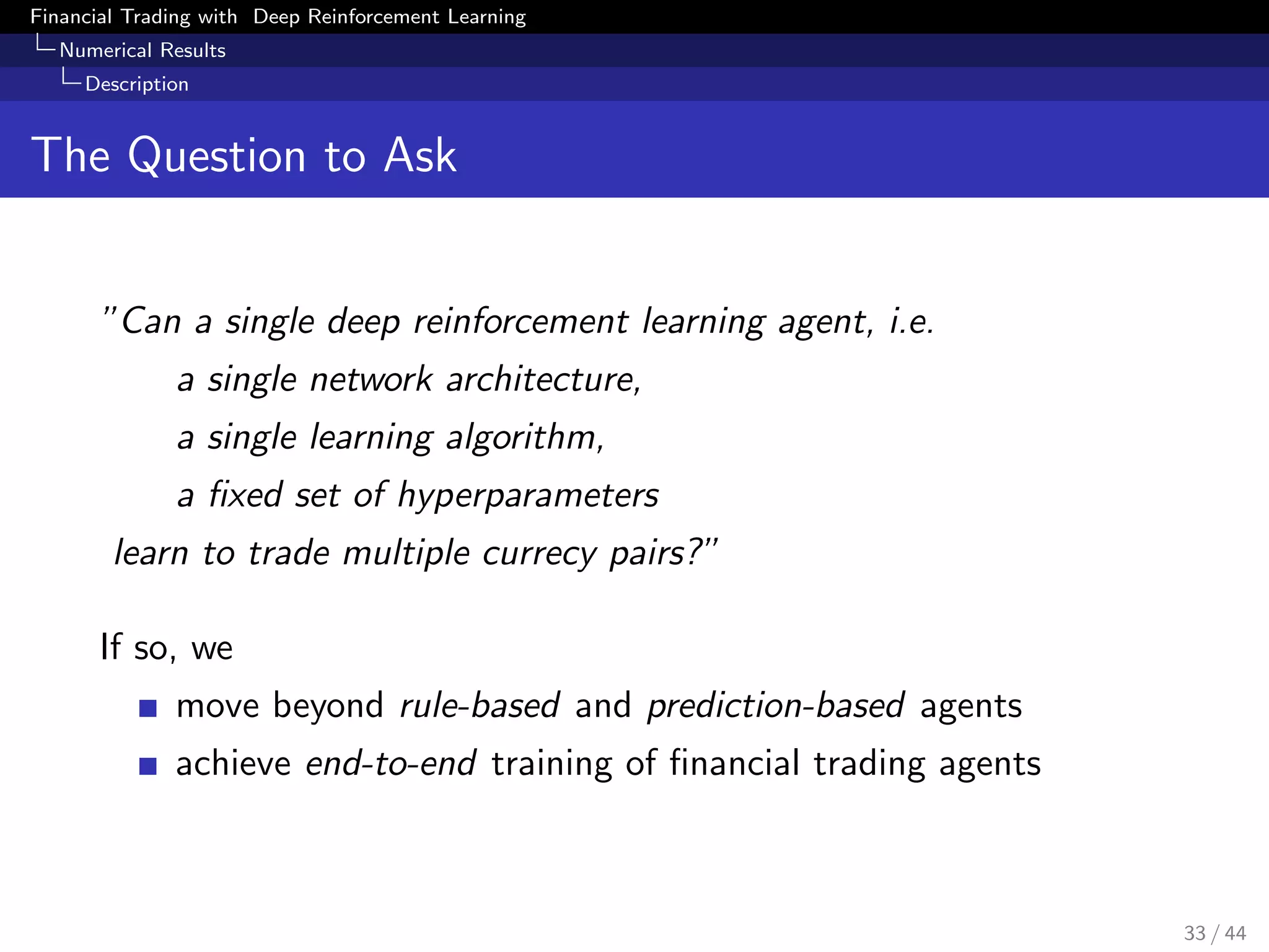
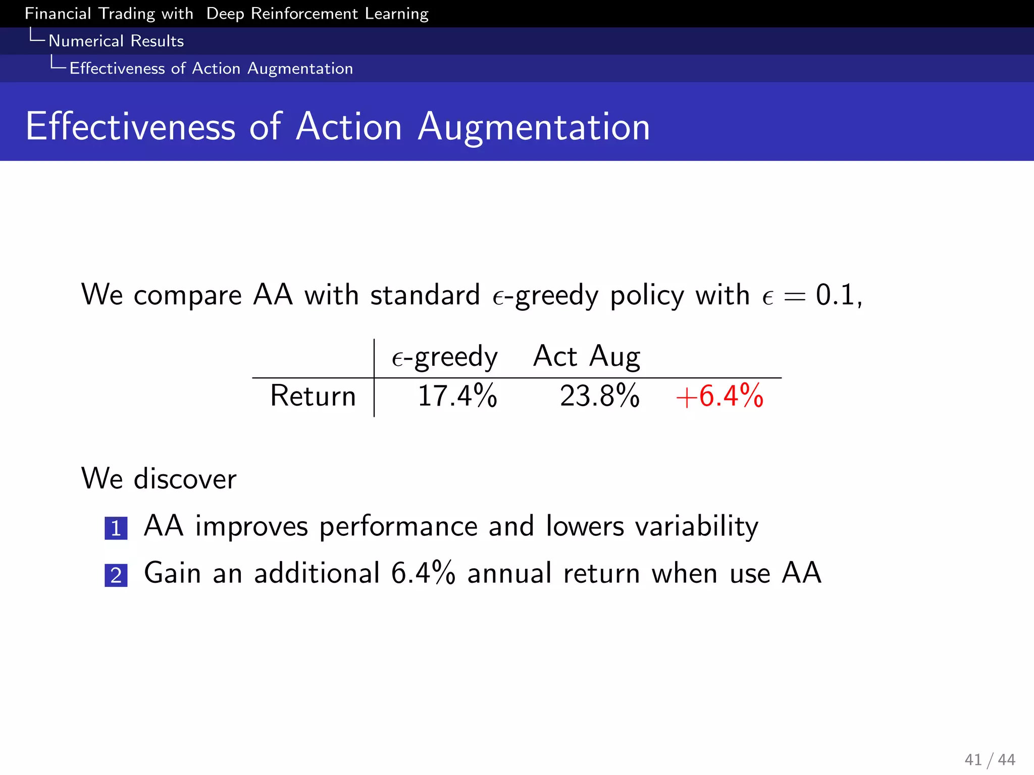
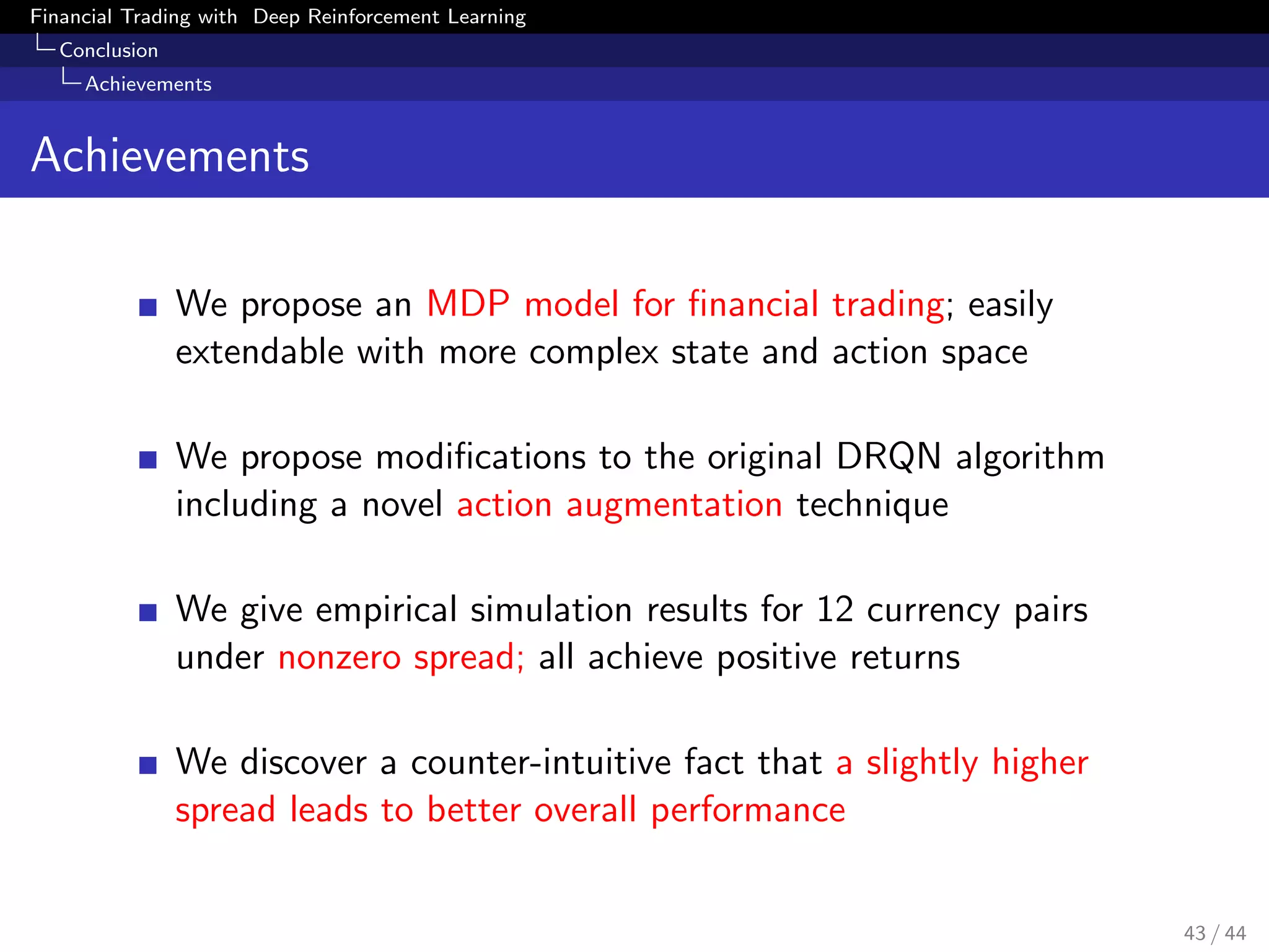
The document discusses financial trading using deep reinforcement learning, detailing methods such as model-free reinforcement learning, Markov decision processes, and the architecture of deep Q-networks. It presents a proposed method that involves data preparation and action augmentation to improve trading strategy, ultimately aiming to determine if a single agent can learn to trade multiple currency pairs. Numerical results are provided to support the effectiveness of the proposed deep reinforcement learning approach in financial trading scenarios.

1. Financial Trading with Deep Reinforcement Learning
Financial Trading with
Deep Reinforcement Learning
Huang, Chien-Yi
cyhuang.am03g@nctu.edu.tw
Dept. of Applied Mathematics, NCTU
July 8, 2018
1 / 44

2. Financial Trading with Deep Reinforcement Learning
Outline
1 Deep Reinforcement Learning
2 Proposed Method
3 Numerical Results
4 Conclusion
2 / 44

3. Financial Trading with Deep Reinforcement Learning
Deep Reinforcement Learning
Outline
1 Deep Reinforcement Learning
2 Proposed Method
3 Numerical Results
4 Conclusion
3 / 44

4. Financial Trading with Deep Reinforcement Learning
Deep Reinforcement Learning
Reinforcement Learning
Model-free Reinforcement Learning
1
Model-free reinforcement learning:
Optimize policy directly; do not build a model for the env.
Learning from scratch through trial-and-error; no supervisor
1
Sutton and Barto. Reinforcement learning: An introduction, 1998
4 / 44

5. Financial Trading with Deep Reinforcement Learning
Deep Reinforcement Learning
Reinforcement Learning
Model-free Reinforcement Learning
1
Model-free reinforcement learning:
Optimize policy directly; do not build a model for the env.
Learning from scratch through trial-and-error; no supervisor
1
Sutton and Barto. Reinforcement learning: An introduction, 1998
5 / 44

6. Financial Trading with Deep Reinforcement Learning
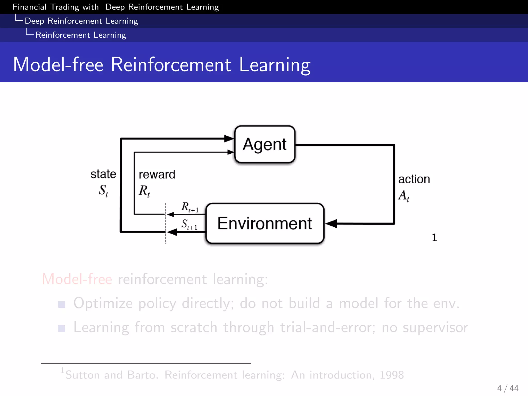
Deep Reinforcement Learning
Markov Decision Process
Markov Decision Process
Definition
A Markov Decision Process is a tuple (S, A, p, r, γ) where
S is a finite set of states
A is a finite set of actions
p is a transition probability distribution,
p(s | s, a) = P [St+1 = s | St = s, At = a]
r is a reward function, r(s, a) = E [Rt+1 | St = s, At = a]
γ ∈ (0, 1) is a discount factor
In real applications of model-free RL, we only define the state
space, action space and reward function
Reward function should reflect the ultimate goal
6 / 44

7. Financial Trading with Deep Reinforcement Learning
Deep Reinforcement Learning
Markov Decision Process
Markov Decision Process
Definition
A Markov Decision Process is a tuple (S, A, p, r, γ) where
S is a finite set of states
A is a finite set of actions
p is a transition probability distribution,
p(s | s, a) = P [St+1 = s | St = s, At = a]
r is a reward function, r(s, a) = E [Rt+1 | St = s, At = a]
γ ∈ (0, 1) is a discount factor
In real applications of model-free RL, we only define the state
space, action space and reward function
Reward function should reflect the ultimate goal
7 / 44

8. Financial Trading with Deep Reinforcement Learning
Deep Reinforcement Learning
Markov Decision Process
Markov Decision Process
Definition
A Markov Decision Process is a tuple (S, A, p, r, γ) where
S is a finite set of states
A is a finite set of actions
p is a transition probability distribution,
p(s | s, a) = P [St+1 = s | St = s, At = a]
r is a reward function, r(s, a) = E [Rt+1 | St = s, At = a]
γ ∈ (0, 1) is a discount factor
In real applications of model-free RL, we only define the state
space, action space and reward function
Reward function should reflect the ultimate goal
8 / 44

9. Financial Trading with Deep Reinforcement Learning
Deep Reinforcement Learning
Definition and Theorem
Return and Policy
Definition
The return Gt is the total sum of discounted rewards from time
step t,
Gt = Rt+1 + γRt+2 + γ2
Rt+3 + · · · =
∞
k=0
γk
Rt+k+1
Definition
A policy π is a distribution over actions given states,
π(a|s) = P[At = a | St = s]
9 / 44

10. Financial Trading with Deep Reinforcement Learning
Deep Reinforcement Learning
Definition and Theorem
Return and Policy
Definition
The return Gt is the total sum of discounted rewards from time
step t,
Gt = Rt+1 + γRt+2 + γ2
Rt+3 + · · · =
∞
k=0
γk
Rt+k+1
Definition
A policy π is a distribution over actions given states,
π(a|s) = P[At = a | St = s]
10 / 44

11. Financial Trading with Deep Reinforcement Learning
Deep Reinforcement Learning
Definition and Theorem
Value Function
Definition
The action-value function Qπ(s, a) of an MDP is the expected
return starting from state s, taking action a and then following
policy π,
Qπ
(s, a) = Eπ[Gt | St = s, At = a]
Definition
The optimal action-value function Q∗(s, a) is the maximum value
function over all policies
Q∗
(s, a) = max
π
Qπ
(s, a)
11 / 44

12. Financial Trading with Deep Reinforcement Learning
Deep Reinforcement Learning
Definition and Theorem
Value Function
Definition
The action-value function Qπ(s, a) of an MDP is the expected
return starting from state s, taking action a and then following
policy π,
Qπ
(s, a) = Eπ[Gt | St = s, At = a]
Definition
The optimal action-value function Q∗(s, a) is the maximum value
function over all policies
Q∗
(s, a) = max
π
Qπ
(s, a)
12 / 44

13. Financial Trading with Deep Reinforcement Learning
Deep Reinforcement Learning
Definition and Theorem
Bellman Equation
Theorem
Optimal value function satisfies Bellman Optimality Equation,
Q∗
(s, a) = E[Rt+1 + γ max
a
Q∗
(St+1, a ) | St = s, At = a]
1 Once we have Q∗, we can act optimally,
π∗
(s) = arg max
a
Q∗
(s, a)
2 Cannot compute expectation without environment dynamics
3 Sample the Bellman equation through interaction with env
13 / 44

14. Financial Trading with Deep Reinforcement Learning
Deep Reinforcement Learning
Definition and Theorem
Bellman Equation
Theorem
Optimal value function satisfies Bellman Optimality Equation,
Q∗
(s, a) = E[Rt+1 + γ max
a
Q∗
(St+1, a ) | St = s, At = a]
1 Once we have Q∗, we can act optimally,
π∗
(s) = arg max
a
Q∗
(s, a)
2 Cannot compute expectation without environment dynamics
3 Sample the Bellman equation through interaction with env
14 / 44

15. Financial Trading with Deep Reinforcement Learning
Deep Reinforcement Learning
Definition and Theorem
Bellman Equation
Theorem
Optimal value function satisfies Bellman Optimality Equation,
Q∗
(s, a) = E[Rt+1 + γ max
a
Q∗
(St+1, a ) | St = s, At = a]
1 Once we have Q∗, we can act optimally,
π∗
(s) = arg max
a
Q∗
(s, a)
2 Cannot compute expectation without environment dynamics
3 Sample the Bellman equation through interaction with env
15 / 44

16. Financial Trading with Deep Reinforcement Learning
Deep Reinforcement Learning
Q-Learning and Deep Q-Network (DQN)
Q-Learning1
Goal: learn Q∗ for an MDP
Every step, perform an incremental update on Q(s, a),
Q(s, a) ← Q(s, a) + α (r + γ max
a
Q(s , a )
Q-target
−Q(s, a))
Guarantee convergence with proper step-size schedule
Tabular method does not scale up to large problems
1
Watkins and Dayan. Q-learning (1992)
16 / 44

17. Financial Trading with Deep Reinforcement Learning
Deep Reinforcement Learning
Q-Learning and Deep Q-Network (DQN)
Deep Q-Network1
Parametrize Q∗ with deep neural network Qθ, e.g. CNN
Target network Qθ− :
A delayed version of Qθ to compute the target value
Q-target ≡ r + γ max
a
Qθ− (s , a )
Soft update on target network θ−
← τθ + (1 − τ)θ−
Experience replay:
Store previous transitions to a replay memory D
Sample a mini-batch from D for training each step
Train network Qθ with mean square loss and gradient descent
L(θ) = E(s,a,r,s )∼D (r + γ max
a
Qθ− (s , a ) − Qθ(s, a))2
θ ← θ − α θL(θ)
1
Mnih et al. Playing atari with deep reinforcement learning (2013)
17 / 44

18. Financial Trading with Deep Reinforcement Learning
Deep Reinforcement Learning
Modifications to DQN
Modifications to DQN
1 Double Q-Learning and Double DQN1
Overestimation in Q-Learning
Use the online network to pick the argmax
Q-target ≡ r + γQθ− (s , arg max
a
Qθ(s , a ))
2 Deep Recurrent Q-Network (DRQN)2
Add an additional LSTM layer before output layer
Sample a sequence instead of a minibatch; train with BPTT
1
Van Hasselt et al. Deep Reinforcement Learning with Double Q-Learning. (2016)
2
Hausknecht et al. Deep recurrent q-learning for partially observable mdps (2015)
18 / 44

19. Financial Trading with Deep Reinforcement Learning
Deep Reinforcement Learning
Modifications to DQN
Modifications to DQN
1 Double Q-Learning and Double DQN1
Overestimation in Q-Learning
Use the online network to pick the argmax
Q-target ≡ r + γQθ− (s , arg max
a
Qθ(s , a ))
2 Deep Recurrent Q-Network (DRQN)2
Add an additional LSTM layer before output layer
Sample a sequence instead of a minibatch; train with BPTT
1
Van Hasselt et al. Deep Reinforcement Learning with Double Q-Learning. (2016)
2
Hausknecht et al. Deep recurrent q-learning for partially observable mdps (2015)
19 / 44

20. Financial Trading with Deep Reinforcement Learning
Proposed Method
Outline
1 Deep Reinforcement Learning
2 Proposed Method
3 Numerical Results
4 Conclusion
20 / 44

21. Financial Trading with Deep Reinforcement Learning
Proposed Method
Data Preparation
Data Preparation
Source TrueFX.com
Type tick-by-tick data
Symbol 12 currency pairs1
Duration from 2012.01 to 2017.12
Timeframe 15-minute interval
Data open, high, low, close prices and tick volume
Post-processing intersect time indices for alignment
Size after post processing: 139813
1
AUDJPY, AUDNZD, AUDUSD, CADJPY, CHFJPY, EURGBP, EURJPY, EURUSD, GBPJP, GBPUSD,
NZDUSD, USDCAD
21 / 44

22. Financial Trading with Deep Reinforcement Learning
Proposed Method
MDP Formulation
State, Action and Reward
State ∈ R198
Sinusoidal encoding of minute, hour, day of week ∈ R3
Recent 8 lag log returns on close for all symbols ∈ R8×12
Recent 8 lag log returns on volume for all symbols ∈ R8×12
One-hot encoding of current position ∈ R3
Agent’s memory: last hidden state ht−1 in LSTM layer
Action ∈ R3
Position to hold at next time step ∈ {−1, 0, 1}
Position reversal is allowed
Reward
One-step portfolio log return, rt = log( vt
vt−1
)
22 / 44

23. Financial Trading with Deep Reinforcement Learning
Proposed Method
MDP Formulation
State, Action and Reward
State ∈ R198
Sinusoidal encoding of minute, hour, day of week ∈ R3
Recent 8 lag log returns on close for all symbols ∈ R8×12
Recent 8 lag log returns on volume for all symbols ∈ R8×12
One-hot encoding of current position ∈ R3
Agent’s memory: last hidden state ht−1 in LSTM layer
Action ∈ R3
Position to hold at next time step ∈ {−1, 0, 1}
Position reversal is allowed
Reward
One-step portfolio log return, rt = log( vt
vt−1
)
23 / 44

24. Financial Trading with Deep Reinforcement Learning
Proposed Method
MDP Formulation
State, Action and Reward
State ∈ R198
Sinusoidal encoding of minute, hour, day of week ∈ R3
Recent 8 lag log returns on close for all symbols ∈ R8×12
Recent 8 lag log returns on volume for all symbols ∈ R8×12
One-hot encoding of current position ∈ R3
Agent’s memory: last hidden state ht−1 in LSTM layer
Action ∈ R3
Position to hold at next time step ∈ {−1, 0, 1}
Position reversal is allowed
Reward
One-step portfolio log return, rt = log( vt
vt−1
)
24 / 44

25. Financial Trading with Deep Reinforcement Learning
Proposed Method
Model Architecture
Model Architecture
Q(St )
ht−1 ht · · ·
•
•
St
output
LSTM
hidden
hidden
Layer 4 Linear layer with 3 units
Layer 3 LSTM layer with 256 units
Layer 2 Linear layer with 256 units
ELU activation1
Layer 1 Linear layer with 256 units
ELU activation
Layer 0 State St (input)
Model size ≈ 65k parameters
1
Clevert et al. Fast and accurate deep network learning by exponential linear units (elus) (2015)
25 / 44

26. Financial Trading with Deep Reinforcement Learning
Proposed Method
Action Augmentation
Action Augementation
Random exploration is unsatisfying in financial trading
E.g. -greedy,
π(a|s) =
/|A| + 1 − if a∗
= arg maxa Q(s, a)
/|A| otherwise
Action augmentation:
We can compute reward signal for all actions
The successor state only differs by agent’s position
Enrich the feedback signal to the agent
Encode prior knowledge in learning
A novel loss function to incorporate action augmentation,
we update Q-value for all actions
L(θ) = E(s,a,r,s )∼D r + γQθ− (s , arg max
a
Qθ(s , a )) − Qθ(s, a) 2
26 / 44

27. Financial Trading with Deep Reinforcement Learning
Proposed Method
Action Augmentation
Action Augementation
Random exploration is unsatisfying in financial trading
E.g. -greedy,
π(a|s) =
/|A| + 1 − if a∗
= arg maxa Q(s, a)
/|A| otherwise
Action augmentation:
We can compute reward signal for all actions
The successor state only differs by agent’s position
Enrich the feedback signal to the agent
Encode prior knowledge in learning
A novel loss function to incorporate action augmentation,
we update Q-value for all actions
L(θ) = E(s,a,r,s )∼D r + γQθ− (s , arg max
a
Qθ(s , a )) − Qθ(s, a) 2
27 / 44

28. Financial Trading with Deep Reinforcement Learning
Proposed Method
Action Augmentation
Action Augementation
Random exploration is unsatisfying in financial trading
E.g. -greedy,
π(a|s) =
/|A| + 1 − if a∗
= arg maxa Q(s, a)
/|A| otherwise
Action augmentation:
We can compute reward signal for all actions
The successor state only differs by agent’s position
Enrich the feedback signal to the agent
Encode prior knowledge in learning
A novel loss function to incorporate action augmentation,
we update Q-value for all actions
L(θ) = E(s,a,r,s )∼D r + γQθ− (s , arg max
a
Qθ(s , a )) − Qθ(s, a) 2
28 / 44

29. Financial Trading with Deep Reinforcement Learning
Proposed Method
Learning Algorithm
Algorithm 1 Financial DRQN Algorithm
Initialize:
T ∈ N, recurrent Q-network Qθ, target network Qθ− ← Qθ, dataset D
Simulate env E from dataset D
step ← 1
Observe initial state s from env E
for each step do
step ← step + 1
Select greedy action w.r.t. Qθ(s, a) and apply to env E
Receive reward r and next state s from env E
Augment actions to form T = (s, a, r, s ) and store T to memory D
if D is filled and step mod T = 0 then
Sample a sequence of length T from D
Train network Qθ with action augmentation loss and BPTT
end if
Soft update target network θ−
← (1 − τ)θ−
+ τθ
end for
29 / 44

30. Financial Trading with Deep Reinforcement Learning
Proposed Method
Learning Algorithm
Summary
Agent consists of
LSTM network (model)
F-DRQN (algorithm)
Agent takes in financial data
Agent actions ∈ {−1, 0, 1}
Agent maximizes portfolio value
30 / 44

31. Financial Trading with Deep Reinforcement Learning
Numerical Results
Outline
1 Deep Reinforcement Learning
2 Proposed Method
3 Numerical Results
4 Conclusion
31 / 44

32. Financial Trading with Deep Reinforcement Learning
Numerical Results
Description
The Question to Ask
”Can a single deep reinforcement learning agent, i.e.
a single network architecture,
a single learning algorithm,
a fixed set of hyperparameters
learn to trade multiple currecy pairs?”
If so, we
move beyond rule-based and prediction-based agents
achieve end-to-end training of financial trading agents
32 / 44

33. Financial Trading with Deep Reinforcement Learning
Numerical Results
Description
The Question to Ask
”Can a single deep reinforcement learning agent, i.e.
a single network architecture,
a single learning algorithm,
a fixed set of hyperparameters
learn to trade multiple currecy pairs?”
If so, we
move beyond rule-based and prediction-based agents
achieve end-to-end training of financial trading agents
33 / 44

34. Financial Trading with Deep Reinforcement Learning
Numerical Results
Simulation Trading
Hyperparameters for Training and Simulation
We use a substantially smaller replay memory
Initial cash in base currency of the pair
Fixed spread if otherwise stated
Training
Learning timestep T 96
Replay memory size N 480
Learning rate 0.00025
Optimizer Adam
Discount factor 0.99
Target network τ 0.001
Simulation
Initial cash 100,000
Trade size 100,000
Spread (bp) 0.08
Trading days 252 days
34 / 44

35. Financial Trading with Deep Reinforcement Learning
Numerical Results
Simulation Trading
Hyperparameters for Training and Simulation
We use a substantially smaller replay memory
Initial cash in base currency of the pair
Fixed spread if otherwise stated
Training
Learning timestep T 96
Replay memory size N 480
Learning rate 0.00025
Optimizer Adam
Discount factor 0.99
Target network τ 0.001
Simulation
Initial cash 100,000
Trade size 100,000
Spread (bp) 0.08
Trading days 252 days
35 / 44

36. Financial Trading with Deep Reinforcement Learning
Numerical Results
Simulation Trading
Simulation Result with Baseline
36 / 44

37. Financial Trading with Deep Reinforcement Learning
Numerical Results
Simulation Trading
Trading Statistics
We compute trading statistics averaging over all symbols,
Win Rate Risk-Reward1 Corr2 Freq
59.8% 0.76 0.12 4.6
Patterns found in trading strategies discovered by the agent,
1 Agent favors strategies with high win rate ≈ 60%
2 Agent favors strategies with lower risk-reward ratio ≈ 0.75
3 Agent discovers strategies with low correlation
4 Agent makes trading decisions roughly every hour
1
average profit divides average loss
2
average absolute correlation with baseline
37 / 44

38. Financial Trading with Deep Reinforcement Learning
Numerical Results
The Effect of Spread
The Effect of Spread
38 / 44

39. Financial Trading with Deep Reinforcement Learning
Numerical Results
The Effect of Spread
The Effect of Spread
Annual return under different spreads,
Spread (bp) 0.08 0.1 0.15 0.2
Return 23.8% 26.3% 16.7% 11.9%
We discover,
1 Wide spread harms performance in general
2 We discover a counter-intuitive fact:
a slightly higher spread leads better overall performance
39 / 44

40. Financial Trading with Deep Reinforcement Learning
Numerical Results
Effectiveness of Action Augmentation
Effectiveness of Action Augmentation
40 / 44

41. Financial Trading with Deep Reinforcement Learning
Numerical Results
Effectiveness of Action Augmentation
Effectiveness of Action Augmentation
We compare AA with standard -greedy policy with = 0.1,
-greedy Act Aug
Return 17.4% 23.8% +6.4%
We discover
1 AA improves performance and lowers variability
2 Gain an additional 6.4% annual return when use AA
41 / 44

42. Financial Trading with Deep Reinforcement Learning
Conclusion
Outline
1 Deep Reinforcement Learning
2 Proposed Method
3 Numerical Results
4 Conclusion
42 / 44

43. Financial Trading with Deep Reinforcement Learning
Conclusion
Achievements
Achievements
We propose an MDP model for financial trading; easily
extendable with more complex state and action space
We propose modifications to the original DRQN algorithm
including a novel action augmentation technique
We give empirical simulation results for 12 currency pairs
under nonzero spread; all achieve positive returns
We discover a counter-intuitive fact that a slightly higher
spread leads to better overall performance
43 / 44

44. Financial Trading with Deep Reinforcement Learning
Conclusion
Future Directions
Future Directions
Expand state and action space,
Macro data, NLP data...
Adjustable position size, limit orders...
Different financial trading setting, e.g. high frequency trading
Different input state and action space
Different reward function
Distributional reinforcement learning:
Q(s, a)
D
= R(s, a) + γQ(S , A )
Pick action with Sharpe ratio
a = arg max
a∈A
E[Q]
Var[Q]
44 / 44