An Introduction to Reinforcement
Learning (RL) and RL Brain Machine
Interface (RL-BMI)


                  Aditya Tarigoppula
                          www.joefrancislab.com
                   SUNY Downstate Medical Center
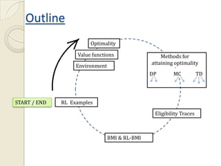
Outline
                        Optimality

                   Value functions                  Methods for
                                                attaining optimality
                   Environment
                                                DP       MC           TD


START / END   RL Examples

                                                 Eligibility Traces


                                 BMI & RL-BMI
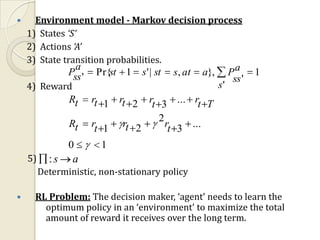
     Environment model - Markov decision process
    1) States ‘S’
    2) Actions ‘A’
    3) State transition probabilities.
                  a
                Pss '    Pr{st 1    s ' | st   s, at   a},        Pa      1
                                                                   ss '
    4) Reward                                                s'
                Rt      rt 1 rt 2   rt 3 ... rt T
                                       2
                Rt      rt 1   rt 2      rt 3 ...
                0         1
    5)     :s    a
         Deterministic, non-stationary policy

    RL Problem: The decision maker, ‘agent’ needs to learn the
       optimum policy in an ‘environment’ to maximize the total
       amount of reward it receives over the long term.
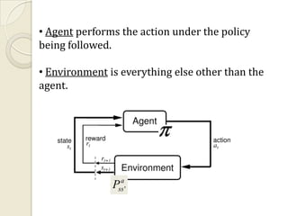
• Agent performs the action under the policy
being followed.

• Environment is everything else other than the
agent.


                 a
               Pss '
Value Functions:
   State Value Function
              V ( s)        E {Rt | st                      s}
                                                  k
                 E {rt      1                         rt   k 2   | st        s}
                                         k 0
                                                 a      a
                        ( s, a )               Pss ' [ Rss '        V ( s ' )]
                  a                       s'


   State – Action Value Function
              Q ( s, a )        E {Rt | st                  s, at        a}
                                k
                E {                 rt   k 1   | st        s, at        a}
                      k 0
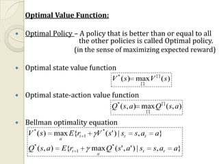
Optimal Value Function:

   Optimal Policy – A policy that is better than or equal to all
                     the other policies is called Optimal policy.
                   (in the sense of maximizing expected reward)

   Optimal state value function
                               V * ( s) maxV ( s)

   Optimal state-action value function
                               Q* ( s, a) max Q ( s, a)

   Bellman optimality equation
     V * ( s) max E{rt 1 V * ( s' ) | st         s, at   a}
                    a

     Q * ( s, a )   E{rt   1   max Q* ( s' , a' ) | st   s, at   a}
                                 a
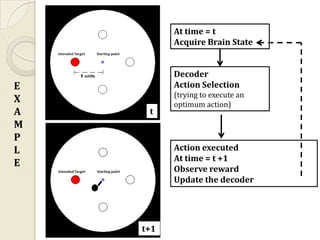
At time = t
          Acquire Brain State


          Decoder
E         Action Selection
          (trying to execute an
X         optimum action)
A    t
M
P
L         Action executed
          At time = t +1
E
          Observe reward
          Update the decoder


    t+1
S1

                            Pr 0.8


E         S3    Pr 0.1                       Pr 0.1     S2
X
A
M                            Pr 0
P                                S4
L
E
    V ( s) [0.8 * ( R( s, a1 )        *V ( s1 )) 0.1* ( R( s, a2 )...
    ...   *V ( s2 )) 0.1* ( R( s, a3 )           *V ( s3 ))]

                                      Prof. Andrew Ng, Lecture
                                      16, Machine learning
Outline
                                                           We're here !
                        Optimality

                   Value functions
                                                    Methods for
                   Environment                  attaining optimality
                                                DP       MC           TD


START / END   RL Examples

                                                 Eligibility Traces


                                 BMI & RL-BMI
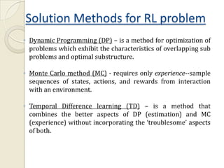
Solution Methods for RL problem
◦ Dynamic Programming (DP) – is a method for optimization of
  problems which exhibit the characteristics of overlapping sub
  problems and optimal substructure.

◦ Monte Carlo method (MC) - requires only experience--sample
  sequences of states, actions, and rewards from interaction
  with an environment.

◦ Temporal Difference learning (TD) – is a method that
  combines the better aspects of DP (estimation) and MC
  (experience) without incorporating the ‘troublesome’ aspects
  of both.
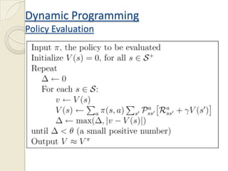
Dynamic Programming
Policy Evaluation
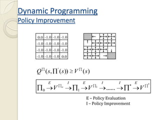
Dynamic Programming
Policy Improvement


                   '
     Q ( s,            ( s )) V ( s )
           E                I       E           I            I       E       *
                                                                 *
       0       V        o
                                1       V   1
                                                    ......               V
                                        E – Policy Evaluation
                                        I – Policy Improvement
Policy Iteration            Value Iteration
D
Y
N
A
M
I
C

P
R
O                                         Replace entire
G                                         section with
R
A                      V (s)   max          a      a
                                          Pss ' [ Rss '   V ( s ' )]
                                a
M                                    s'

M
I
N
G
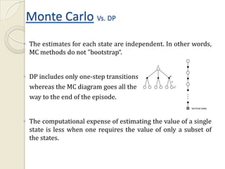
Monte Carlo Vs. DP
◦ The estimates for each state are independent. In other words,
  MC methods do not "bootstrap“.


◦ DP includes only one-step transitions
  whereas the MC diagram goes all the
  way to the end of the episode.


◦ The computational expense of estimating the value of a single
  state is less when one requires the value of only a subset of
  the states.
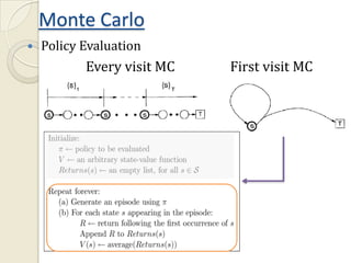
Monte Carlo
   Policy Evaluation
           Every visit MC   First visit MC
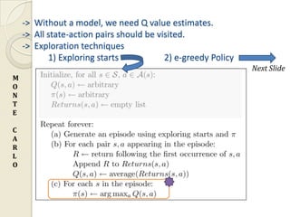
-> Without a model, we need Q value estimates.
    -> All state-action pairs should be visited.
    -> Exploration techniques
           1) Exploring starts            2) e-greedy Policy
                                                               Next Slide
M
O
N
T
E

C
A
R
L
O
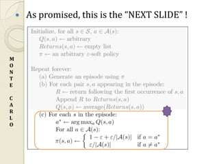
   As promised, this is the “NEXT SLIDE” !


M
O
N
T
E

C
A
R
L
O
Temporal Difference Methods
◦ Like MC, TD methods can learn directly from raw experience
  without a model of the environment's dynamics. Like DP, TD
  methods update estimates are based in part on other learned
  estimates, without waiting for a final outcome (they bootstrap).


  V ( st )   V ( st )   [rt   1   V ( st 1 ) V ( st )]
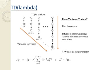
TD(lambda)
                       Bias –Variance Tradeoff


                       Bias decreases


                       Intuition: start with large
                       ‘lamda’ and then decrease
                       over time
  Variance Increases


                         trace decay parameter
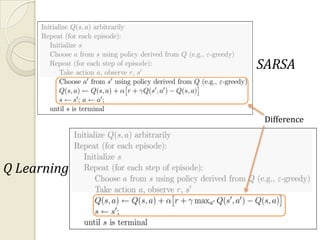
SARSA


              Difference


Q Learning
Outline
                        Optimality

                   Value functions                  Methods for
                                                attaining optimality
                   Environment
                                                DP       MC       TD


START / END   RL Examples

                                                 Eligibility Traces


                                                           We're here !
                                 BMI & RL-BMI
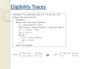
Eligibility Traces


                     OR
Outline
                        Optimality

                   Value functions                  Methods for
                                                attaining optimality
                   Environment
                                                DP        MC           TD


START / END   RL Examples

                                                  Eligibility Traces


                                 BMI & RL-BMI

                                                We're here !
Online/closed loop RL-BMI architecture


NEURAL                                      action         output _ index[max(Qi ( st ))]
SIGNAL
                                            Q( st , at )     Qi ( st , action)


                                                             reward
                      tanh(.)

                                     TD _ err    rt         * Q( st 1 , at 1 ) Q( st , at )
                                     delta TD _ err * e _ trace
         ‘delta’ used for updating
         the weights through
         back-propagation
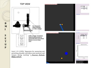
B
M
I

S
E
T
U
P
    Scott, S. H. (1999). "Apparatus for measuring and
    perturbing shoulder and elbow joint positions and
    torques during reaching." J Neurosci Methods
    89(2): 119-27.
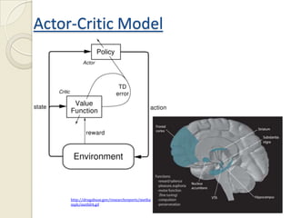
Actor-Critic Model


     http://drugabuse.gov/researchreports/metha
     mph/meth04.gif
References
   Reinforcement Learning: An Introduction
    Richard S. Sutton & Andrew G. Barto
   Prof. Andrew Ng’s machine Learning Lectures
   http://heli.stanford.edu
   Dr. Joseph T. Francis
    www.joefrancislab.com
   Prof. Peter Dayan
   Dr. Justin Sanchez Group
    http://www.bme.miami.edu/nrg/

An introduction to reinforcement learning (rl)

  • 1.
    An Introduction toReinforcement Learning (RL) and RL Brain Machine Interface (RL-BMI) Aditya Tarigoppula www.joefrancislab.com SUNY Downstate Medical Center
  • 2.
    Outline Optimality Value functions Methods for attaining optimality Environment DP MC TD START / END RL Examples Eligibility Traces BMI & RL-BMI
  • 4.
    Environment model - Markov decision process 1) States ‘S’ 2) Actions ‘A’ 3) State transition probabilities. a Pss ' Pr{st 1 s ' | st s, at a}, Pa 1 ss ' 4) Reward s' Rt rt 1 rt 2 rt 3 ... rt T 2 Rt rt 1 rt 2 rt 3 ... 0 1 5) :s a Deterministic, non-stationary policy  RL Problem: The decision maker, ‘agent’ needs to learn the optimum policy in an ‘environment’ to maximize the total amount of reward it receives over the long term.
  • 5.
    • Agent performsthe action under the policy being followed. • Environment is everything else other than the agent. a Pss '
  • 6.
    Value Functions:  State Value Function V ( s) E {Rt | st s} k E {rt 1 rt k 2 | st s} k 0 a a ( s, a ) Pss ' [ Rss ' V ( s ' )] a s'  State – Action Value Function Q ( s, a ) E {Rt | st s, at a} k E { rt k 1 | st s, at a} k 0
  • 7.
    Optimal Value Function:  Optimal Policy – A policy that is better than or equal to all the other policies is called Optimal policy. (in the sense of maximizing expected reward)  Optimal state value function V * ( s) maxV ( s)  Optimal state-action value function Q* ( s, a) max Q ( s, a)  Bellman optimality equation V * ( s) max E{rt 1 V * ( s' ) | st s, at a} a Q * ( s, a ) E{rt 1 max Q* ( s' , a' ) | st s, at a} a
  • 8.
    At time =t Acquire Brain State Decoder E Action Selection (trying to execute an X optimum action) A t M P L Action executed At time = t +1 E Observe reward Update the decoder t+1
  • 9.
    S1 Pr 0.8 E S3 Pr 0.1 Pr 0.1 S2 X A M Pr 0 P S4 L E V ( s) [0.8 * ( R( s, a1 ) *V ( s1 )) 0.1* ( R( s, a2 )... ... *V ( s2 )) 0.1* ( R( s, a3 ) *V ( s3 ))] Prof. Andrew Ng, Lecture 16, Machine learning
  • 10.
    Outline We're here ! Optimality Value functions Methods for Environment attaining optimality DP MC TD START / END RL Examples Eligibility Traces BMI & RL-BMI
  • 11.
    Solution Methods forRL problem ◦ Dynamic Programming (DP) – is a method for optimization of problems which exhibit the characteristics of overlapping sub problems and optimal substructure. ◦ Monte Carlo method (MC) - requires only experience--sample sequences of states, actions, and rewards from interaction with an environment. ◦ Temporal Difference learning (TD) – is a method that combines the better aspects of DP (estimation) and MC (experience) without incorporating the ‘troublesome’ aspects of both.
  • 12.
  • 13.
    Dynamic Programming Policy Improvement ' Q ( s, ( s )) V ( s ) E I E I I E * * 0 V o 1 V 1 ...... V E – Policy Evaluation I – Policy Improvement
  • 14.
    Policy Iteration Value Iteration D Y N A M I C P R O Replace entire G section with R A V (s) max a a Pss ' [ Rss ' V ( s ' )] a M s' M I N G
  • 15.
    Monte Carlo Vs.DP ◦ The estimates for each state are independent. In other words, MC methods do not "bootstrap“. ◦ DP includes only one-step transitions whereas the MC diagram goes all the way to the end of the episode. ◦ The computational expense of estimating the value of a single state is less when one requires the value of only a subset of the states.
  • 16.
    Monte Carlo  Policy Evaluation Every visit MC First visit MC
  • 17.
    -> Without amodel, we need Q value estimates. -> All state-action pairs should be visited. -> Exploration techniques 1) Exploring starts 2) e-greedy Policy Next Slide M O N T E C A R L O
  • 18.
    As promised, this is the “NEXT SLIDE” ! M O N T E C A R L O
  • 19.
    Temporal Difference Methods ◦Like MC, TD methods can learn directly from raw experience without a model of the environment's dynamics. Like DP, TD methods update estimates are based in part on other learned estimates, without waiting for a final outcome (they bootstrap). V ( st ) V ( st ) [rt 1 V ( st 1 ) V ( st )]
  • 20.
    TD(lambda) Bias –Variance Tradeoff Bias decreases Intuition: start with large ‘lamda’ and then decrease over time Variance Increases  trace decay parameter
  • 21.
    SARSA Difference Q Learning
  • 22.
    Outline Optimality Value functions Methods for attaining optimality Environment DP MC TD START / END RL Examples Eligibility Traces We're here ! BMI & RL-BMI
  • 23.
  • 24.
    Outline Optimality Value functions Methods for attaining optimality Environment DP MC TD START / END RL Examples Eligibility Traces BMI & RL-BMI We're here !
  • 25.
    Online/closed loop RL-BMIarchitecture NEURAL action output _ index[max(Qi ( st ))] SIGNAL Q( st , at ) Qi ( st , action) reward tanh(.) TD _ err rt * Q( st 1 , at 1 ) Q( st , at ) delta TD _ err * e _ trace ‘delta’ used for updating the weights through back-propagation
  • 26.
    B M I S E T U P Scott, S. H. (1999). "Apparatus for measuring and perturbing shoulder and elbow joint positions and torques during reaching." J Neurosci Methods 89(2): 119-27.
  • 28.
    Actor-Critic Model http://drugabuse.gov/researchreports/metha mph/meth04.gif
  • 29.
    References  Reinforcement Learning: An Introduction Richard S. Sutton & Andrew G. Barto  Prof. Andrew Ng’s machine Learning Lectures  http://heli.stanford.edu  Dr. Joseph T. Francis www.joefrancislab.com  Prof. Peter Dayan  Dr. Justin Sanchez Group http://www.bme.miami.edu/nrg/

Editor's Notes

  • #2 It receives evaluative signal rather than instructive in nature i.e. no one tells the agent “this is how you do it and point out each and every mistake made” instead agent is told “good work or bad work”…1) RL in nature….US as children or deciding on a cuisine for dinner (past experiences with the cuisine and what is the expectation for reward for all cuisines being considered today), playing chess, learning a new sport etc. 2) The RL agent is trying to learn the manner of interaction with the environment (called Policy) so that it can maximize “reward” or a notion of reward…i.e. it is trying to develop a behavior for a given environment.3) Lets start with what we will be achieving by the end of this talk…..Simulation and video of online RL-BMI
  • #3 We will start here and end back here and hopefully by the end of the talk will be reinforced with reward (in terms of knowledge and some knowledge of RL)
  • #5 Markov chain a model for a random process that evolves over time such that the states (like locations in a maze) occupied in the future are independent of the states in the past given the current state. I.E. CONDITIONAL prob of next state is dependent only the present state and the action taken.Markov decision problem (MDP) a model for a controlled random process in which an agent's choice of action determines the probabilities of transitions of a Markov chain and lead to rewards (or costs) that need to be maximized (or minimized).The environment is modeled as a MDP ( process which is partly random and partly deterministic in nature)...The environment agrees in the Markovian property. A RL task that satisfies the Markov property ( the conditional probability distribution of future states of the process (conditional on both past and present values) depends only upon the present state; that is, given the present, the future does not depend on the past) and it can distinguish between all the states is called MDP. If the agent cannot distinguish between all the available states of the environment then its called partially observable MDP (POMDP). MDP consists of four components S, A, P, R (Show where these components are in the simulation)…if there are finite number of states and actions then it is called finite MDP. The states corresponding to the decision making are observable to the agent (assumption). The action deemed best by the agent is taken which results in the transition into a new state S’talk about state transition probabilities i.e in a given state even if you do decide to move in a particular direction, you can calculate the probabilities of moving from one state to the other. Eg – if I want to move north from where I am standing the probability of reaching 1 step in north is ‘x’ but the probability of reaching Bronx in 1 step is almost equal to zero. OR taking a step forward…6) Explain the cumulative reward for the environment which is an absorbing process i.e. it has a termination state which would result in a next trial…and non terminal trial. i.e. utilization of the discounting factor7) Differentiate between immediate reward (payoff) and the long term reward (payoff).
  • #7 the expected valueof a random variable is the weighted average of all possible values that this random variable can take on.It’s called the Bellman’s Equation.
  • #8 1) Explain how you do you decide if one policy is better than the other using the state value function. 2) Principle of Optimality: An optimal policy has the property that whatever the initial state and initial decision are, the remaining decisions must constitute an optimal policy with regard to the state resulting from the first decision.3) Intuitively, the Bellman optimality equation expresses the fact that the value of a state under an optimal policy must equal the expected return for the best action from that state.
  • #9 Brain state – put the image of spikes
  • #10 Why is DP a good methods for a finite MDP with a relatively manageable dimensionality (states) wherein the dynamics of the environment is completely known ? Explain how if you knew everything about the environment’s dynamics then you end up with a system of linear equations wherein the number of linear equations and the number of unknowns ends up being the same and thus we can sole it to get the value function for all the states given a policy which is being evaluated. (grid example with different probabilities and calculation of V)  and  denote the number of states and actions, this means that a DP method takes a number of computational operations that is less than some polynomial function of  and . A DP method is guaranteed to find an optimal policy in polynomial time even though the total number of (deterministic) policies is . In this sense, DP is exponentially faster than any direct search in policy space could be, because direct search would have to exhaustively examine each policy to provide the same guarantee.DP algorithms are obtained by turning Bellman equations into iterative assignment statements (update rule). To deal with higher dimensional states structure, we can use asynchronous DP. (you might just not state anything about this).
  • #12 http://20bits.com/articles/introduction-to-dynamic-programming/In Monte Carlo, you usually perform a task and update your policy once you
  • #13 Policy evaluation is also called as Prediction problem.
  • #14 As seen in Policy evaluation you will calculate the value functions for each state for a given policy. But in order to find an optimal policy you would have to perform sweeps over all possible policies available. An easier way to modify the current policy in an environment whose dynamics are completely known and DP is being used to find the optimum policy would be to use policy improvement along with policy evaluation. At this point the policy after each improvement can be seen as a greedy policy.
  • #15 The greedy policy takes the action that looks best in the short term--after one step of lookahead--according to . By construction, the greedy policy meets the conditions of the policy improvement theorem (4.7), so we know that it is as good as, or better than, the original policy. The process of making a new policy that improves on an original policy, by making it greedy with respect to the value function of the original policy, is called policy improvement.
  • #16 http://www.cs.wmich.edu/~trenary/files/cs5300/RLBook/node51.htmlIf DP had feelings, then right now it would be feeling sad….its like saying here’s my first child…he can do all this awesome stuff but here is my second son who can do all these awesome stuff but at a faster rate !! Imagine what it will do to DP when I talk about TD techniques….it will just crush them !! Bootstrap - estimate for one state does not build upon the estimate of any other state, as is the case in DP
  • #18 Generalized Policy Iteration - In GPI one maintains both an approximate policy and an approximate value function. The value function is repeatedly altered to more closely approximate the value function for the current policy, and the policy is repeatedly improved with respect to the current value function:If a model is not available, then it is particularly useful to estimate action values rather than state values. With a model, state values alone are sufficient to determine a policy; one simply looks ahead one step and chooses whichever action leads to the best combination of reward and next state, as we did in the chapter on DP. Without a model, however, state values alone are not sufficient. One must explicitly estimate the value of each action in order for the values to be useful in suggesting a policy. Thus, one of our primary goals for Monte Carlo methods is to estimate Q*. To achieve this, we first consider another policy evaluation problem.The policy evaluation problem for action values is to estimate Q(pi)(s,a) , the expected return when starting in state s , taking action a , and thereafter following policy . The Monte Carlo methods here are essentially the same as just presented for state values.
  • #20 1) In effect, the target for the Monte Carlo update is R(t), whereas the target for the TD update is r(t+1) + gamma*V(s).2) Becausethe TD method bases its update in part on an existing estimate, we say that it is a bootstrapping  method, like DP
  • #24 http://www.cs.wmich.edu/~trenary/files/cs5300/RLBook/node75.htmlhttp://www.cs.wmich.edu/~trenary/files/cs5300/RLBook/node80.htmlThere are two ways to view eligibility traces. The more theoretical view, which we emphasize here, is that they are a bridge from TD to Monte Carlo methods. When TD methods are augmented with eligibility traces, they produce a family of methods spanning a spectrum that has Monte Carlo methods at one end and one-step TD methods at the other. In between are intermediate methods that are often better than either extreme method. In this sense eligibility traces unify TD and Monte Carlo methods in a valuable and revealing way.The other way to view eligibility traces is more mechanistic. From this perspective, an eligibility trace is a temporary record of the occurrence of an event, such as the visiting of a state or the taking of an action. The trace marks the memory parameters associated with the event as eligible for undergoing learning changes. When a TD error occurs, only the eligible states or actions are assigned credit or blame for the error. Thus, eligibility traces help bridge the gap between events and training information. Like TD methods themselves, eligibility traces are a basic mechanism for temporal credit assignment.
  • #25 http://cs.rochester.edu/~kautz/Courses/290Bspring2008/NeuroRobots/TiNS_2006.pdf
  • #29 Actor-critic methods are TD methods that have a separate memory structure to explicitly represent the policy independent of the value function. The policy structure is known as the actor, because it is used to select actions, and the estimated value function is known as the critic, because it criticizes the actions made by the actor.