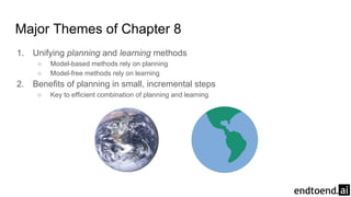
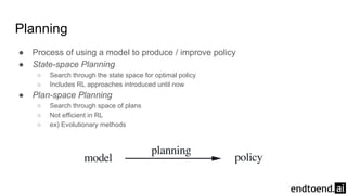
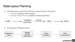
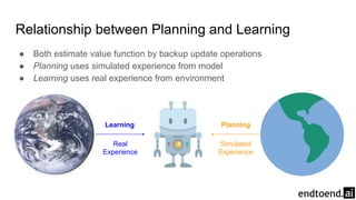
Chapter 8: Planning and Learning with
Tabular Methods
Seungjae Ryan Lee
Major Themes of Chapter 8
1. Unifying planning and learning methods
○ Model-based methods rely on planning
○ Model-free methods rely on learning
2. Benefits of planning in small, incremental steps
○ Key to efficient combination of planning and learning
Model of the Environment
● Anything the agent can use to predict the environment
● Used to mimic or simulate experience
1. Distribution models
○ Describe all possibilities and probabilities
○ Stronger but difficult to obtain
2. Sample models
○ Produce one possibility sampled according to the probabilities
○ Weaker but easier to obtain
Planning
● Process of using a model to produce / improve policy
● State-space Planning
○ Search through the state space for optimal policy
○ Includes RL approaches introduced until now
● Plan-space Planning
○ Search through space of plans
○ Not efficient in RL
○ ex) Evolutionary methods
State-space Planning
● All state-space planning methods share common structure
○ Involves computing value functions
○ Compute value functions by updates or backup operations
● ex) Dynamic Programming
Distribution
model
Sweeps
through
state space
Policy
Evaluation
Policy
Improvement
Relationship between Planning and Learning
● Both estimate value function by backup update operations
● Planning uses simulated experience from model
● Learning uses real experience from environment
Learning Planning
Real
Experience
Simulated
Experience
Random-sample one-step tabular Q-planning
● Planning and Learning is similar enough to transfer algorithms
● Same convergence guarantees as one-step tabular Q-learning
○ All states and actions selected infinitely many times
○ Step size decrease over time
● Need just the sample model
Random-sample one-step tabular Q-planning
On-line Planning
● Need to incorporate new experience with planning
● Divide computational resources between decision making and model learning
Roles of Real Experience
1. Model learning: Improve the model to increase accuracy
2. Direct RL: Directly improve the value function and policy
Direct Reinforcement Learning
● Improve value functions and policy with real experience
● Simpler and not affected by bias from model design
Indirect Reinforcement Learning
● Improve value functions and policy by improving the model
● Achieve better policy with fewer environmental interactions
Dyna-Q
● Simple on-line planning agent with all processes
○ Planning: random-sample one-step tabular Q-planning
○ Direct RL: one-step tabular Q-learning
○ Model learning: Return last observed next state and reward as prediction
Dyna-Q: Implementation
● Order of process on a serial computer
● Can be parallelized to a reactive, deliberative agent
○ reactive: responding instantly to latest information
○ deliberative: always planning in the background
● Planning is most computationally intensive
○ Complete n iteration of Q-planning algorithm on each timestep
Acting Direct RL
Model
Learning
Planning
Dyna-Q: Pseudocode
Acting
Direct RL
Model Learning
Planning
Dyna Maze Example
● Only reward is on reaching goal state (+1)
○ Takes long time for reward propagate
Dyna Maze Example: Result
● Much faster convergence to optimal policy
Dyna Maze Example: Intuition
● Without planning, each episode adds only one step to the policy
● With planning, extensive policy is developed by the end of episode
Black square : location of the agent
Halfway through second episode
Possibility of a Wrong Model
● Model can be wrong for various reasons:
○ Stochastic environment & limited number of samples
○ Function approximation
○ Environment has changed
● Can lead to suboptimal policy
Optimistic Wrong Model: Blocking Maze Example
● Agent can correct modelling error for optimistic models
○ Agent attempts to “exploit” false opportunities
○ Agent discovers they do not exist
Environment changes after 1000 timesteps
Optimistic Wrong Model: Blocking Maze Example
(Ignore Dyna-Q+ for now)
Pessimistic Wrong Model: Shortcut Maze Example
● Agent might never learn modelling error for optimistic models
○ Agent never realizes a better path exists
○ Unlikely even with an ε-greedy policy
Environment changes after 1000 timesteps
Pessimistic Wrong Model: Shortcut Maze Example
(Ignore Dyna-Q+ for now)
Dyna-Q+
● Need to balance exploration and exploitation
● Keep track of elapsed time since last visit for each state-action pair
● Add bonus reward during planning
● Allow untried state-action pair to be visited in planning
● Costly, but the computational curiosity is worth the cost
Prioritized Sweeping: Intuition
● Focused simulated transitions and updates can make planning more efficient
○ At the start of second episode, only the penultimate state has nonzero value estimate
○ Almost updates do nothing
Prioritized Sweeping: Backward Focusing
● Intuition: work backward from “goal states”
● Work back from any state whose value changed
○ Typically implies other states’ values also changed
● Update predecessor states of changed state
V(s’) = -1
a
s
V(s’) = -1
a
s
Prioritized Sweeping
● Not all changes are equally useful
○ magnitude of change in value
○ transition probabilities
● Prioritize updates via priority queue
○ Pop max-priority pair and update
○ Insert all predecessor pairs with effect above some small threshold
■ (Only keep higher priority if already exists)
○ Repeat until quiescence
Prioritized Sweeping: Pseudocode
Prioritized Sweeping: Maze Example
● Decisive advantage over unprioritized Dyna-Q
Prioritized Sweeping: Rod Maneuvering Example
● Maneuver rod around obstacles
○ 14400 potential states, 4 actions (translate, rotate)
● Too large to be solved without prioritization
Prioritized Sweeping: Limitations
● Stochastic environment
○ Use expected update instead of sample updates
○ Can waste computation on low-probability transitions
● How about sample updates?
Expected vs Sample Updates
● Recurring theme throughout RL
● Any can be used for planning
Expected vs Sample Updates
● Expected updates yields better estimate
● Sample updates requires less computation
Expected vs Sample Updates: Computation
● Branching factor d: number of possible next states
○ Determines computation needed for expected update
○ T(Expected update) ≈ d * T(Sample update)
● If enough time for expected update, resulting estimate is usually better
○ No sampling error
● If not enough time, sample update can at least somewhat improve estimate
○ Smaller steps
Expected vs Sample Updates: Analysis
● Sample updates reduce error according to
● Does not account sample update having better estimate of successor states
Distributing Updates
1. Dynamic Programming
○ Sweep through entire state space (or state-action space)
2. Dyna-Q
○ Sample uniformly
● Both suffers from updating irrelevant states most of the time
Trajectory Sampling
● Gather experience by sampling explicit individual trajectories
○ Sample state transitions and rewards from the model
○ Sample actions from a distribution
● Effects of on-policy distribution
○ Can ignore vast, uninteresting parts of the space
○ Significantly advantageous when function approximation is used
S1 S2 S3
R2 = +1 R3 = -1
Model ModelPolicy Policy Policy
Trajectory Sampling: On-policy Distribution Example
● Faster planning initially, but retarded in the long run
● Better when branching factor b is small (can focus on just few states)
Trajectory Sampling: On-policy Distribution Example
● Long-lasting advantage when state space is large
○ Focusing on states have bigger impact when state space is large
Real-time Dynamic Programming (RTDP)
● On-policy trajectory-sampling value iteration algorithm
● Gather real or simulated trajectories
○ Asynchronous DP: nonsystematic sweeps
● Update with value iteration
S1 S2 S3
R2 = +1 R3 = -1
Model ModelPolicy Policy Policy
RTDP: Prediction and Control
● Prediction problem: skip any state not reachable by policy
● Control problem: find the optimal partial policy
○ A policy that is optimal for relevant states but arbitrary for other states
○ Finding such policy requires visiting all (s, a) infinitely many times
Stochastic Optimal Path Problems
● Conditions
○ Undiscounted episodic task with absorbing goal states
○ Initial value of every goal state is 0
○ At least one policy can definitively reach a goal state from any starting state
○ All rewards from non-goal states are negative
○ All initial values are optimistic
● Guarantees
○ RTDP does not need to visit all (s, a) infinite times to find optimal partial policy
Stochastic Optimal Path Problem: Racetrack
● 9115 reachable states, 599 relevant
● RTDP needs half the update of DP
○ Visits almost all states at least once
○ Focuses to relevant states quickly
DP vs. RTDP: Checking Convergence
● DP: Update with exhaustive sweeps until Δv is sufficiently small
○ Unaware of policy performance until value function has converged
○ Could lead to overcomputation
● RTDP: Update with trajectories
○ Check policy performance via trajectories
○ Detect convergence earlier than DP
● Background Planning
○ Gradually improve policy or value function
○ Not focused on the current state
○ Better when low-latency action selection is required
● Decision-Time Planning
○ Select single action through planning
○ Focused on the current state
○ Typically discard value / policy used in planning after each action selection
○ Most useful when fast responses are not required
Background Planning vs. Decision-Time Planning
Heuristic Search
● Generate tree of possible continuations for each encountered states
○ Compute best action with the search tree
○ More computation is needed
○ Slower response time
● Value function can be held constant or updated
● Works best with perfect model and imperfect Q
Heuristic Search: Focusing States
● Focus on states that might immediate follow the current state
○ Computations: Generate tree with current state as head
○ Memory: Store estimates only for relevant states
● Particularly efficient when state space is large (ex. chess)
Heuristic Search: Focusing Updates
● Focus distribution of updates on the current state
○ Construct search tree
○ Perform one-step updates from bottom-up
Rollout Algorithms
● Estimate Q by averaging simulated trajectories from a rollout policy
● Choose action with highest Q
● Does not compute Q for all states / actions (unlike MC control)
● Not a learning algorithm since values and policies are not stored
http://www.wbc.poznan.pl/Content/351255/Holfeld_Denise_Simroth_Axel_A_Monte_Carlo_Rollout_algorithm_for_stock_control.pdf
● Satisfies the policy improvement theorem for the policy
○ Same as one step of the policy iteration algorithm
● Rollout seeks to improve upon the default policy, not to find the optimal policy
○ Better default policy → Better estimates → Better policy from rollout algorithm
Rollout Algorithms: Policy
● Good rollout policies need a lot of trajectories
● Rollout algorithms often have strict time constraints
Possible Mitigations
1. Run trajectories on separate processors
2. Truncate simulated trajectories before termination
○ Use stored evaluation function
3. Prune unlikely candidate actions
Rollout Algorithms: Time Constraints
Monte Carlo Tree Search (MCTS)
● Rollout algorithm with directed simulations
○ Accumulate value estimates in a tree structure
○ Direct simulations toward more high-rewarding trajectories
● Behind successes in Go
Monte Carlo Tree Search: Algorithm
● Repeat until termination:
a. Selection: Select beginning of trajectory
b. Expansion: Expand tree
c. Simulation: Simulate an episode
d. Backup: Update values
● Select action with some criteria
a. Largest action value
b. Largest visit count
Monte Carlo Tree Search: Selection
● Start at the root node
● Traverse down the tree to select a leaf node
Monte Carlo Tree Search: Expansion
● Expand the selected leaf node
○ Add one or more child nodes via unexplored actions
Monte Carlo Tree Search: Simulation
● From leaf node or new child node, simulate a complete episode
● Generates a Monte Carlo trial
○ Selected first by the tree policy
○ Selected beyond the tree by the rollout policy
Monte Carlo Tree Search: Backup
● Update or Initialize values of nodes traversed in tree policy
○ No values saved for the rollout policy beyond the tree
https://en.wikipedia.org/wiki/Monte_Carlo_tree_search
Monte Carlo Tree Search: Insight
● Can use online, incremental, sample-based methods
● Can focus MC trials on segments with high-return trajectories
● Can efficiently grow a partial value table
○ Does not need to save all values
○ Does not need function approximation
Summary of Chapter 8
● Planning requires a model of the environment
○ Distribution model consists of transition probabilities
○ Sample model produces single transitions and rewards
● Planning and Learning share many similarities
○ Any learning method can be converted to planning method
● Planning can vary in size of updates
○ ex) 1-step sample updates
● Planning can vary in distribution of updates
○ ex) Prioritized sweeping, On-policy trajectory sampling, RTDP
● Planning can focus forward from pertinent states
○ Decision-time planning
○ ex) Heuristic search, Rollout algorithms, MCTS
Summary of Part I
● Three underlying ideas:
a. Estimate value functions
b. Back up values along actual / possible state trajectories
c. Use Generalized Policy Iteration (GPI)
■ Keep approximate value function and policy
■ Use one to improve another
Summary of Part I: Dimensions
● Three important dimensions:
a. Sample update vs Expected update
■ Sample update: Using a sample trajectory
■ Expected update: Using the distribution model
b. Depth of updates: degree of bootstrapping
c. On-policy vs Off-policy methods
● One undiscussed important dimension:
Function Approximation
Summary of Part I: Other Dimensions
● Episodic vs. Continuing returns
● Discounted vs. Undiscounted returns
● Action values vs. State values vs. Afterstate values
● Exploration methods
○ ε-greedy, optimistic initialization, softmax, UCB
● Synchronous vs. Asynchronous updates
● Real vs. Simulated experience
● Location, Timing, and Memory of updates
○ Which state or state-action pair to update in model-based methods?
○ Should updates be part of selected actions, or only afterward?
○ How long should the updated values be retained?
Thank you!
Original content from
● Reinforcement Learning: An Introduction by Sutton and Barto
You can find more content in
● github.com/seungjaeryanlee
● www.endtoend.ai

Reinforcement Learning 8: Planning and Learning with Tabular Methods

  • 1.
    Chapter 8: Planningand Learning with Tabular Methods Seungjae Ryan Lee
  • 2.
    Major Themes ofChapter 8 1. Unifying planning and learning methods ○ Model-based methods rely on planning ○ Model-free methods rely on learning 2. Benefits of planning in small, incremental steps ○ Key to efficient combination of planning and learning
  • 3.
    Model of theEnvironment ● Anything the agent can use to predict the environment ● Used to mimic or simulate experience 1. Distribution models ○ Describe all possibilities and probabilities ○ Stronger but difficult to obtain 2. Sample models ○ Produce one possibility sampled according to the probabilities ○ Weaker but easier to obtain
  • 4.
    Planning ● Process ofusing a model to produce / improve policy ● State-space Planning ○ Search through the state space for optimal policy ○ Includes RL approaches introduced until now ● Plan-space Planning ○ Search through space of plans ○ Not efficient in RL ○ ex) Evolutionary methods
  • 5.
    State-space Planning ● Allstate-space planning methods share common structure ○ Involves computing value functions ○ Compute value functions by updates or backup operations ● ex) Dynamic Programming Distribution model Sweeps through state space Policy Evaluation Policy Improvement
  • 6.
    Relationship between Planningand Learning ● Both estimate value function by backup update operations ● Planning uses simulated experience from model ● Learning uses real experience from environment Learning Planning Real Experience Simulated Experience
  • 7.
    Random-sample one-step tabularQ-planning ● Planning and Learning is similar enough to transfer algorithms ● Same convergence guarantees as one-step tabular Q-learning ○ All states and actions selected infinitely many times ○ Step size decrease over time ● Need just the sample model
  • 8.
  • 9.
    On-line Planning ● Needto incorporate new experience with planning ● Divide computational resources between decision making and model learning
  • 10.
    Roles of RealExperience 1. Model learning: Improve the model to increase accuracy 2. Direct RL: Directly improve the value function and policy
  • 11.
    Direct Reinforcement Learning ●Improve value functions and policy with real experience ● Simpler and not affected by bias from model design
  • 12.
    Indirect Reinforcement Learning ●Improve value functions and policy by improving the model ● Achieve better policy with fewer environmental interactions
  • 13.
    Dyna-Q ● Simple on-lineplanning agent with all processes ○ Planning: random-sample one-step tabular Q-planning ○ Direct RL: one-step tabular Q-learning ○ Model learning: Return last observed next state and reward as prediction
  • 14.
    Dyna-Q: Implementation ● Orderof process on a serial computer ● Can be parallelized to a reactive, deliberative agent ○ reactive: responding instantly to latest information ○ deliberative: always planning in the background ● Planning is most computationally intensive ○ Complete n iteration of Q-planning algorithm on each timestep Acting Direct RL Model Learning Planning
  • 15.
  • 16.
    Dyna Maze Example ●Only reward is on reaching goal state (+1) ○ Takes long time for reward propagate
  • 17.
    Dyna Maze Example:Result ● Much faster convergence to optimal policy
  • 18.
    Dyna Maze Example:Intuition ● Without planning, each episode adds only one step to the policy ● With planning, extensive policy is developed by the end of episode Black square : location of the agent Halfway through second episode
  • 19.
    Possibility of aWrong Model ● Model can be wrong for various reasons: ○ Stochastic environment & limited number of samples ○ Function approximation ○ Environment has changed ● Can lead to suboptimal policy
  • 20.
    Optimistic Wrong Model:Blocking Maze Example ● Agent can correct modelling error for optimistic models ○ Agent attempts to “exploit” false opportunities ○ Agent discovers they do not exist Environment changes after 1000 timesteps
  • 21.
    Optimistic Wrong Model:Blocking Maze Example (Ignore Dyna-Q+ for now)
  • 22.
    Pessimistic Wrong Model:Shortcut Maze Example ● Agent might never learn modelling error for optimistic models ○ Agent never realizes a better path exists ○ Unlikely even with an ε-greedy policy Environment changes after 1000 timesteps
  • 23.
    Pessimistic Wrong Model:Shortcut Maze Example (Ignore Dyna-Q+ for now)
  • 24.
    Dyna-Q+ ● Need tobalance exploration and exploitation ● Keep track of elapsed time since last visit for each state-action pair ● Add bonus reward during planning ● Allow untried state-action pair to be visited in planning ● Costly, but the computational curiosity is worth the cost
  • 25.
    Prioritized Sweeping: Intuition ●Focused simulated transitions and updates can make planning more efficient ○ At the start of second episode, only the penultimate state has nonzero value estimate ○ Almost updates do nothing
  • 26.
    Prioritized Sweeping: BackwardFocusing ● Intuition: work backward from “goal states” ● Work back from any state whose value changed ○ Typically implies other states’ values also changed ● Update predecessor states of changed state V(s’) = -1 a s V(s’) = -1 a s
  • 27.
    Prioritized Sweeping ● Notall changes are equally useful ○ magnitude of change in value ○ transition probabilities ● Prioritize updates via priority queue ○ Pop max-priority pair and update ○ Insert all predecessor pairs with effect above some small threshold ■ (Only keep higher priority if already exists) ○ Repeat until quiescence
  • 28.
  • 29.
    Prioritized Sweeping: MazeExample ● Decisive advantage over unprioritized Dyna-Q
  • 30.
    Prioritized Sweeping: RodManeuvering Example ● Maneuver rod around obstacles ○ 14400 potential states, 4 actions (translate, rotate) ● Too large to be solved without prioritization
  • 31.
    Prioritized Sweeping: Limitations ●Stochastic environment ○ Use expected update instead of sample updates ○ Can waste computation on low-probability transitions ● How about sample updates?
  • 32.
    Expected vs SampleUpdates ● Recurring theme throughout RL ● Any can be used for planning
  • 33.
    Expected vs SampleUpdates ● Expected updates yields better estimate ● Sample updates requires less computation
  • 34.
    Expected vs SampleUpdates: Computation ● Branching factor d: number of possible next states ○ Determines computation needed for expected update ○ T(Expected update) ≈ d * T(Sample update) ● If enough time for expected update, resulting estimate is usually better ○ No sampling error ● If not enough time, sample update can at least somewhat improve estimate ○ Smaller steps
  • 35.
    Expected vs SampleUpdates: Analysis ● Sample updates reduce error according to ● Does not account sample update having better estimate of successor states
  • 36.
    Distributing Updates 1. DynamicProgramming ○ Sweep through entire state space (or state-action space) 2. Dyna-Q ○ Sample uniformly ● Both suffers from updating irrelevant states most of the time
  • 37.
    Trajectory Sampling ● Gatherexperience by sampling explicit individual trajectories ○ Sample state transitions and rewards from the model ○ Sample actions from a distribution ● Effects of on-policy distribution ○ Can ignore vast, uninteresting parts of the space ○ Significantly advantageous when function approximation is used S1 S2 S3 R2 = +1 R3 = -1 Model ModelPolicy Policy Policy
  • 38.
    Trajectory Sampling: On-policyDistribution Example ● Faster planning initially, but retarded in the long run ● Better when branching factor b is small (can focus on just few states)
  • 39.
    Trajectory Sampling: On-policyDistribution Example ● Long-lasting advantage when state space is large ○ Focusing on states have bigger impact when state space is large
  • 40.
    Real-time Dynamic Programming(RTDP) ● On-policy trajectory-sampling value iteration algorithm ● Gather real or simulated trajectories ○ Asynchronous DP: nonsystematic sweeps ● Update with value iteration S1 S2 S3 R2 = +1 R3 = -1 Model ModelPolicy Policy Policy
  • 41.
    RTDP: Prediction andControl ● Prediction problem: skip any state not reachable by policy ● Control problem: find the optimal partial policy ○ A policy that is optimal for relevant states but arbitrary for other states ○ Finding such policy requires visiting all (s, a) infinitely many times
  • 42.
    Stochastic Optimal PathProblems ● Conditions ○ Undiscounted episodic task with absorbing goal states ○ Initial value of every goal state is 0 ○ At least one policy can definitively reach a goal state from any starting state ○ All rewards from non-goal states are negative ○ All initial values are optimistic ● Guarantees ○ RTDP does not need to visit all (s, a) infinite times to find optimal partial policy
  • 43.
    Stochastic Optimal PathProblem: Racetrack ● 9115 reachable states, 599 relevant ● RTDP needs half the update of DP ○ Visits almost all states at least once ○ Focuses to relevant states quickly
  • 44.
    DP vs. RTDP:Checking Convergence ● DP: Update with exhaustive sweeps until Δv is sufficiently small ○ Unaware of policy performance until value function has converged ○ Could lead to overcomputation ● RTDP: Update with trajectories ○ Check policy performance via trajectories ○ Detect convergence earlier than DP
  • 45.
    ● Background Planning ○Gradually improve policy or value function ○ Not focused on the current state ○ Better when low-latency action selection is required ● Decision-Time Planning ○ Select single action through planning ○ Focused on the current state ○ Typically discard value / policy used in planning after each action selection ○ Most useful when fast responses are not required Background Planning vs. Decision-Time Planning
  • 46.
    Heuristic Search ● Generatetree of possible continuations for each encountered states ○ Compute best action with the search tree ○ More computation is needed ○ Slower response time ● Value function can be held constant or updated ● Works best with perfect model and imperfect Q
  • 47.
    Heuristic Search: FocusingStates ● Focus on states that might immediate follow the current state ○ Computations: Generate tree with current state as head ○ Memory: Store estimates only for relevant states ● Particularly efficient when state space is large (ex. chess)
  • 48.
    Heuristic Search: FocusingUpdates ● Focus distribution of updates on the current state ○ Construct search tree ○ Perform one-step updates from bottom-up
  • 49.
    Rollout Algorithms ● EstimateQ by averaging simulated trajectories from a rollout policy ● Choose action with highest Q ● Does not compute Q for all states / actions (unlike MC control) ● Not a learning algorithm since values and policies are not stored http://www.wbc.poznan.pl/Content/351255/Holfeld_Denise_Simroth_Axel_A_Monte_Carlo_Rollout_algorithm_for_stock_control.pdf
  • 50.
    ● Satisfies thepolicy improvement theorem for the policy ○ Same as one step of the policy iteration algorithm ● Rollout seeks to improve upon the default policy, not to find the optimal policy ○ Better default policy → Better estimates → Better policy from rollout algorithm Rollout Algorithms: Policy
  • 51.
    ● Good rolloutpolicies need a lot of trajectories ● Rollout algorithms often have strict time constraints Possible Mitigations 1. Run trajectories on separate processors 2. Truncate simulated trajectories before termination ○ Use stored evaluation function 3. Prune unlikely candidate actions Rollout Algorithms: Time Constraints
  • 52.
    Monte Carlo TreeSearch (MCTS) ● Rollout algorithm with directed simulations ○ Accumulate value estimates in a tree structure ○ Direct simulations toward more high-rewarding trajectories ● Behind successes in Go
  • 53.
    Monte Carlo TreeSearch: Algorithm ● Repeat until termination: a. Selection: Select beginning of trajectory b. Expansion: Expand tree c. Simulation: Simulate an episode d. Backup: Update values ● Select action with some criteria a. Largest action value b. Largest visit count
  • 54.
    Monte Carlo TreeSearch: Selection ● Start at the root node ● Traverse down the tree to select a leaf node
  • 55.
    Monte Carlo TreeSearch: Expansion ● Expand the selected leaf node ○ Add one or more child nodes via unexplored actions
  • 56.
    Monte Carlo TreeSearch: Simulation ● From leaf node or new child node, simulate a complete episode ● Generates a Monte Carlo trial ○ Selected first by the tree policy ○ Selected beyond the tree by the rollout policy
  • 57.
    Monte Carlo TreeSearch: Backup ● Update or Initialize values of nodes traversed in tree policy ○ No values saved for the rollout policy beyond the tree
  • 59.
  • 60.
    Monte Carlo TreeSearch: Insight ● Can use online, incremental, sample-based methods ● Can focus MC trials on segments with high-return trajectories ● Can efficiently grow a partial value table ○ Does not need to save all values ○ Does not need function approximation
  • 61.
    Summary of Chapter8 ● Planning requires a model of the environment ○ Distribution model consists of transition probabilities ○ Sample model produces single transitions and rewards ● Planning and Learning share many similarities ○ Any learning method can be converted to planning method ● Planning can vary in size of updates ○ ex) 1-step sample updates ● Planning can vary in distribution of updates ○ ex) Prioritized sweeping, On-policy trajectory sampling, RTDP ● Planning can focus forward from pertinent states ○ Decision-time planning ○ ex) Heuristic search, Rollout algorithms, MCTS
  • 62.
    Summary of PartI ● Three underlying ideas: a. Estimate value functions b. Back up values along actual / possible state trajectories c. Use Generalized Policy Iteration (GPI) ■ Keep approximate value function and policy ■ Use one to improve another
  • 63.
    Summary of PartI: Dimensions ● Three important dimensions: a. Sample update vs Expected update ■ Sample update: Using a sample trajectory ■ Expected update: Using the distribution model b. Depth of updates: degree of bootstrapping c. On-policy vs Off-policy methods ● One undiscussed important dimension: Function Approximation
  • 64.
    Summary of PartI: Other Dimensions ● Episodic vs. Continuing returns ● Discounted vs. Undiscounted returns ● Action values vs. State values vs. Afterstate values ● Exploration methods ○ ε-greedy, optimistic initialization, softmax, UCB ● Synchronous vs. Asynchronous updates ● Real vs. Simulated experience ● Location, Timing, and Memory of updates ○ Which state or state-action pair to update in model-based methods? ○ Should updates be part of selected actions, or only afterward? ○ How long should the updated values be retained?
  • 65.
    Thank you! Original contentfrom ● Reinforcement Learning: An Introduction by Sutton and Barto You can find more content in ● github.com/seungjaeryanlee ● www.endtoend.ai