Session Two

  Forecasting
Learning objectives


∗   Define and understand forecasting
∗   Identify the different types of forecasts
∗   Identify and discuss the various time horizons
∗   Discuss different approaches to forecasting
∗   Determine the steps in the forecasting process
∗   Describe and solve averaging techniques in
    forecasting
Learning objectives (cont.)


∗   Solve simple moving average problems
∗   Solve exponential smoothing problems
∗   Determine what constitutes a good forecast
∗   Compare qualitative and quantitative forecasting
    methods.
2.1 Introduction
∗ Forecasting =
  ∗   Preface to planning
  ∗   Attempt to predict future value of a changing variable
  ∗   Subjective or objective
  ∗   Addresses:
      ∗   Macro-circumstances
      ∗   Competitiveness
      ∗   Market tendencies
      ∗   Sourcing funds required.
Examples of Forecasts
Management Information Services – could predict new technology, eg.
Advances in internet

Human Resources – could answer the question “will there be a need
to employ more people in the future
Goods and service design – needs of the customer in the
future
Finance – need for capital replacement, cash flows,
budgets

Operations – scheduling, inventory planning, labour
requirements, and project management

Marketing – prices for new products, promotional
plans, competition analysis
2.2 The uses of forecasts


∗   Plan the system as a whole (long-range)
∗   Plan the use of the system
∗   Business forecasting (predict demand)
∗   Forecasting is never an exact science
∗   Context determines choice of method.
2.3 Features common to all forecasts
∗   Assumption that past trends will be present in future
∗   No precise prediction can be made
∗   Groups more accurate
∗   Longer time horizon is less reliable.
2.4 Time horizons for doing forecasts

∗ Short-range (few weeks – 12 months)
  ∗ More accurate
∗ Medium-range (12 months – 5 years)
∗ Long-range (5 years +)
∗ Medium and long-range: deal with organisation as a whole.
2.4 Time horizons for doing forecasts
                    (cont.)
                Time Horizon    Accuracy          Frequency    Management   Method
                                                               Level


  PROCESS         Long term         Medium            Single       Top      Qual or Quan
   DESIGN
  CAPACITY        Long term         Medium            Single       Top      Qual or Quan
  PLANNING
 AGGREGATE       Medium term         High             Few         Middle    Casual or time
 PLANNING*                                                                      series
 SCHEDULING       Short term       Very high          Many        Lower      Time series

INVENTORY M/      Short term       Very high          Many        Lower      Time series
    MENT


* Capacity planning for medium term 3-18 months
2.5 Requirements of an accurate forecast

∗   Use simple technique
∗   Accuracy
∗   Cost effectiveness
∗   Meaningful units
∗   Timely
∗   Reliable
∗   Should be in writing.
2.6 Forecasting steps


Figure 2.3
2.7 Important situational factors to be
                 considered
∗ Accuracy and cost – trade off between accuracy and cost
∗ Availability of data – large pool of data and relevant
∗ Time span – the longer it is the less accurate it is
∗ Nature of the goods and services – life cycle, seasonal
  variations
∗ Changes in the market - difficult for new products
∗ Use or decision factors – method used and subject should
  be closely related
2.8 Reasons for ineffective forecasts
 ∗ Failure to select applicable model
 ∗ Inability to recognise that forecasting must form an integral
   part of the business
 ∗ Neglecting to monitor the accuracy of the forecast
 ∗ Failure to involve all of the relevant people
 ∗ Inability to realise that the forecast will be wrong
 ∗ Forecasting of incorrect items is not helpful.
2.9 Approaches to forecasting

∗ Qualitative – mainly judgments of the parties involved
∗ Quantitative – calculations & statistical techniques
∗ Associative forecasting techniques – use of equations that
  are descriptive of the variables used. A variable is a factor
  that will influence the composition of a forecast eg. Price of
  product, weather etc
2.9 Approaches to forecasting

∗ Categories of forecasting techniques:
  ∗ Associative methods – equations that
    describe the variables
  ∗ Judgmental forecasts – rely on subjective
    judgment of an individual
  ∗ Time series forecasts – data is manipulated
    using mathematical techniques
2.9 Approaches to forecasting
∗ Qualitative approach:
  ∗ Relied upon when hard data not available
  ∗ Used when forecast required in a hurry
  ∗ Approaches:
    ∗ Consumer surveys – very expensive, validity questionable
    ∗ Jury of executive opinion – top level managers, long term
      forecast
    ∗ Sales-force opinion – grassroots method, very questionable
    ∗ Delphi method – respondents outside company
    ∗ Educated guess – personal insight. Highly unreliable
    ∗ Historical analogy – only if a similar product exists
2.9 Approaches to forecasting (cont.)

 ∗ Quantitative approach:
   ∗ Time series data – use of historical data. Assumes future can be
     based on history
   ∗ Trends – upward or downward movement
   ∗ Seasonality – mostly regular
   ∗ Cycles – e.g. stock market indicators
   ∗ Irregular variations – e.g. flood. Never include in a forecast
   ∗ Random variations – no logical explanation
2.9 Approaches to forecasting (cont.)
2.9 Approaches to forecasting
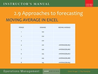
MOVING AVERAGE IN EXCEL
     PERIOD   DEMAND      MOVING AVERAGE

       1       100

       2       250

       3       220

       4       210        =AVERAGE(B2:B5)

       5       240        =AVERAGE(B3:B6)

       6       255        =AVERAGE(B4:B7)

       7       245        =AVERAGE(B5:B8)

       8       195        =AVERAGE(B6:B9)
2.9 Approaches to forecasting

∗ Quantitative techniques:
  ∗   Averaging techniques – the weighted moving average
  ∗   Very similar to moving average technique
  ∗   Moving average gives equal weight to all data
  ∗   Weighted moving average gives different weight to each data
2.9 Weighted Moving Average
Month          Sales ( ‘000)   3 period MA
January        240
February       250
March          230
April          220             (0.5 x 230)+ (0.3 x 250) + (0.2 x 240) = 238
May            270             (0.5 x 220)+ (0.3 x 230) + (0.2 x 250) = 229
June           250             (0.5 x 270)+ (0.3 x 220) + (0.2 x 230) = 247
July           255             (0.5 x 250)+ (0.3 x 270) + (0.2 x 220) = 250
2.9 Problems with Moving Average

 Longer MA period the more smoothed. Forecast less sensitive
  to real fluctuations
 MA does not identify any trends in the data. Time lag +/- 2
  months
 Extensive records of past history must be available
 Weight allocated is arbitrary – trial and error needed
2.9 Approaches to forecasting
∗ Quantitative techniques:
  ∗   Averaging techniques – exponential smoothing
  ∗   Well accepted because
  ∗   Calculations to test accuracy are easy
  ∗   Technique easy to understand
  ∗   Accuracy high for amount of effort required
  ∗   Only small amounts of historical data needed
  ∗   Requires fewer calculations to reach the same answer as other
      methods
2.9 Exponential Smoothing
∗ Predicted 142000 units period 1
∗ Actual 153000 units period 1
∗ α =0.2

Demand period 2 = 142000+0.2(153000-142000) = 144200units
2.9 Approaches to forecasting
∗ Associative forecasting techniques
  ∗ The simple linear regression metho
  ∗ Most widely used method
  ∗ Try to find a linear relationship between two variables
Summary
∗   Defined forecasting
∗   Defined business forecasting
∗   Common features
∗   Requirements
∗   Steps
∗   Situational factors
∗   Reasons for ineffective forecasts
∗   Approaches to forecasting.
For Next Week
∗ Read pages 37 -66 Operations Management
∗ Prepare 1 paragraph discussing the use of forecasts
∗ Prepare 1 paragraph discussing the reasons for
  ineffective forecasts.

Ops management lecture 2 forecasting

  • 1.
    Session Two Forecasting
  • 2.
    Learning objectives ∗ Define and understand forecasting ∗ Identify the different types of forecasts ∗ Identify and discuss the various time horizons ∗ Discuss different approaches to forecasting ∗ Determine the steps in the forecasting process ∗ Describe and solve averaging techniques in forecasting
  • 3.
    Learning objectives (cont.) ∗ Solve simple moving average problems ∗ Solve exponential smoothing problems ∗ Determine what constitutes a good forecast ∗ Compare qualitative and quantitative forecasting methods.
  • 4.
    2.1 Introduction ∗ Forecasting= ∗ Preface to planning ∗ Attempt to predict future value of a changing variable ∗ Subjective or objective ∗ Addresses: ∗ Macro-circumstances ∗ Competitiveness ∗ Market tendencies ∗ Sourcing funds required.
  • 5.
    Examples of Forecasts ManagementInformation Services – could predict new technology, eg. Advances in internet Human Resources – could answer the question “will there be a need to employ more people in the future Goods and service design – needs of the customer in the future Finance – need for capital replacement, cash flows, budgets Operations – scheduling, inventory planning, labour requirements, and project management Marketing – prices for new products, promotional plans, competition analysis
  • 6.
    2.2 The usesof forecasts ∗ Plan the system as a whole (long-range) ∗ Plan the use of the system ∗ Business forecasting (predict demand) ∗ Forecasting is never an exact science ∗ Context determines choice of method.
  • 7.
    2.3 Features commonto all forecasts ∗ Assumption that past trends will be present in future ∗ No precise prediction can be made ∗ Groups more accurate ∗ Longer time horizon is less reliable.
  • 8.
    2.4 Time horizonsfor doing forecasts ∗ Short-range (few weeks – 12 months) ∗ More accurate ∗ Medium-range (12 months – 5 years) ∗ Long-range (5 years +) ∗ Medium and long-range: deal with organisation as a whole.
  • 9.
    2.4 Time horizonsfor doing forecasts (cont.) Time Horizon Accuracy Frequency Management Method Level PROCESS Long term Medium Single Top Qual or Quan DESIGN CAPACITY Long term Medium Single Top Qual or Quan PLANNING AGGREGATE Medium term High Few Middle Casual or time PLANNING* series SCHEDULING Short term Very high Many Lower Time series INVENTORY M/ Short term Very high Many Lower Time series MENT * Capacity planning for medium term 3-18 months
  • 10.
    2.5 Requirements ofan accurate forecast ∗ Use simple technique ∗ Accuracy ∗ Cost effectiveness ∗ Meaningful units ∗ Timely ∗ Reliable ∗ Should be in writing.
  • 11.
  • 12.
    2.7 Important situationalfactors to be considered ∗ Accuracy and cost – trade off between accuracy and cost ∗ Availability of data – large pool of data and relevant ∗ Time span – the longer it is the less accurate it is ∗ Nature of the goods and services – life cycle, seasonal variations ∗ Changes in the market - difficult for new products ∗ Use or decision factors – method used and subject should be closely related
  • 13.
    2.8 Reasons forineffective forecasts ∗ Failure to select applicable model ∗ Inability to recognise that forecasting must form an integral part of the business ∗ Neglecting to monitor the accuracy of the forecast ∗ Failure to involve all of the relevant people ∗ Inability to realise that the forecast will be wrong ∗ Forecasting of incorrect items is not helpful.
  • 14.
    2.9 Approaches toforecasting ∗ Qualitative – mainly judgments of the parties involved ∗ Quantitative – calculations & statistical techniques ∗ Associative forecasting techniques – use of equations that are descriptive of the variables used. A variable is a factor that will influence the composition of a forecast eg. Price of product, weather etc
  • 15.
    2.9 Approaches toforecasting ∗ Categories of forecasting techniques: ∗ Associative methods – equations that describe the variables ∗ Judgmental forecasts – rely on subjective judgment of an individual ∗ Time series forecasts – data is manipulated using mathematical techniques
  • 16.
    2.9 Approaches toforecasting ∗ Qualitative approach: ∗ Relied upon when hard data not available ∗ Used when forecast required in a hurry ∗ Approaches: ∗ Consumer surveys – very expensive, validity questionable ∗ Jury of executive opinion – top level managers, long term forecast ∗ Sales-force opinion – grassroots method, very questionable ∗ Delphi method – respondents outside company ∗ Educated guess – personal insight. Highly unreliable ∗ Historical analogy – only if a similar product exists
  • 17.
    2.9 Approaches toforecasting (cont.) ∗ Quantitative approach: ∗ Time series data – use of historical data. Assumes future can be based on history ∗ Trends – upward or downward movement ∗ Seasonality – mostly regular ∗ Cycles – e.g. stock market indicators ∗ Irregular variations – e.g. flood. Never include in a forecast ∗ Random variations – no logical explanation
  • 18.
    2.9 Approaches toforecasting (cont.)
  • 19.
    2.9 Approaches toforecasting MOVING AVERAGE IN EXCEL PERIOD DEMAND MOVING AVERAGE 1 100 2 250 3 220 4 210 =AVERAGE(B2:B5) 5 240 =AVERAGE(B3:B6) 6 255 =AVERAGE(B4:B7) 7 245 =AVERAGE(B5:B8) 8 195 =AVERAGE(B6:B9)
  • 20.
    2.9 Approaches toforecasting ∗ Quantitative techniques: ∗ Averaging techniques – the weighted moving average ∗ Very similar to moving average technique ∗ Moving average gives equal weight to all data ∗ Weighted moving average gives different weight to each data
  • 21.
    2.9 Weighted MovingAverage Month Sales ( ‘000) 3 period MA January 240 February 250 March 230 April 220 (0.5 x 230)+ (0.3 x 250) + (0.2 x 240) = 238 May 270 (0.5 x 220)+ (0.3 x 230) + (0.2 x 250) = 229 June 250 (0.5 x 270)+ (0.3 x 220) + (0.2 x 230) = 247 July 255 (0.5 x 250)+ (0.3 x 270) + (0.2 x 220) = 250
  • 22.
    2.9 Problems withMoving Average  Longer MA period the more smoothed. Forecast less sensitive to real fluctuations  MA does not identify any trends in the data. Time lag +/- 2 months  Extensive records of past history must be available  Weight allocated is arbitrary – trial and error needed
  • 23.
    2.9 Approaches toforecasting ∗ Quantitative techniques: ∗ Averaging techniques – exponential smoothing ∗ Well accepted because ∗ Calculations to test accuracy are easy ∗ Technique easy to understand ∗ Accuracy high for amount of effort required ∗ Only small amounts of historical data needed ∗ Requires fewer calculations to reach the same answer as other methods
  • 24.
  • 25.
    2.9 Exponential Smoothing ∗Predicted 142000 units period 1 ∗ Actual 153000 units period 1 ∗ α =0.2 Demand period 2 = 142000+0.2(153000-142000) = 144200units
  • 26.
    2.9 Approaches toforecasting ∗ Associative forecasting techniques ∗ The simple linear regression metho ∗ Most widely used method ∗ Try to find a linear relationship between two variables
  • 27.
    Summary ∗ Defined forecasting ∗ Defined business forecasting ∗ Common features ∗ Requirements ∗ Steps ∗ Situational factors ∗ Reasons for ineffective forecasts ∗ Approaches to forecasting.
  • 28.
    For Next Week ∗Read pages 37 -66 Operations Management ∗ Prepare 1 paragraph discussing the use of forecasts ∗ Prepare 1 paragraph discussing the reasons for ineffective forecasts.