Downloaded 24 times

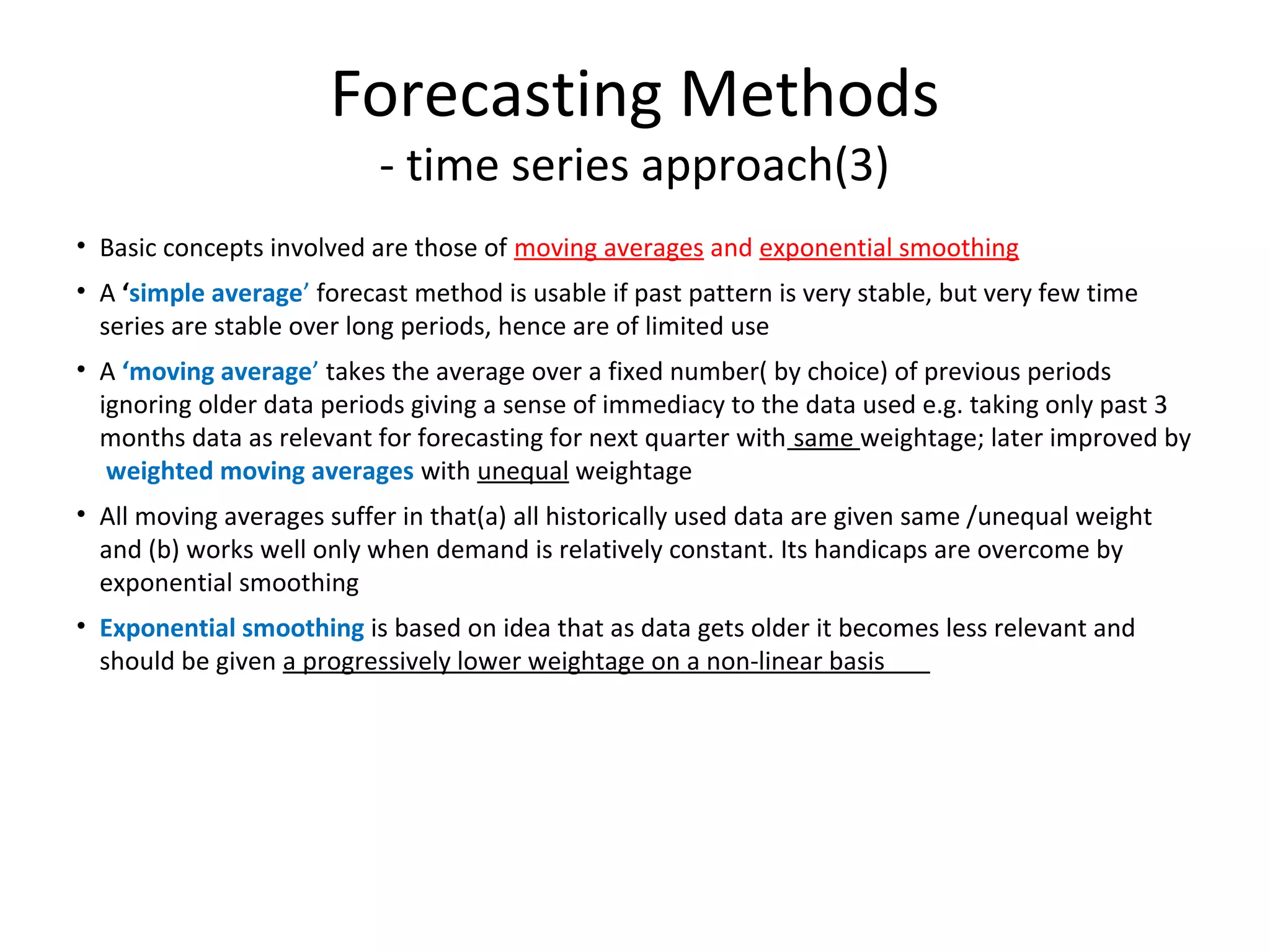
![Static Methods
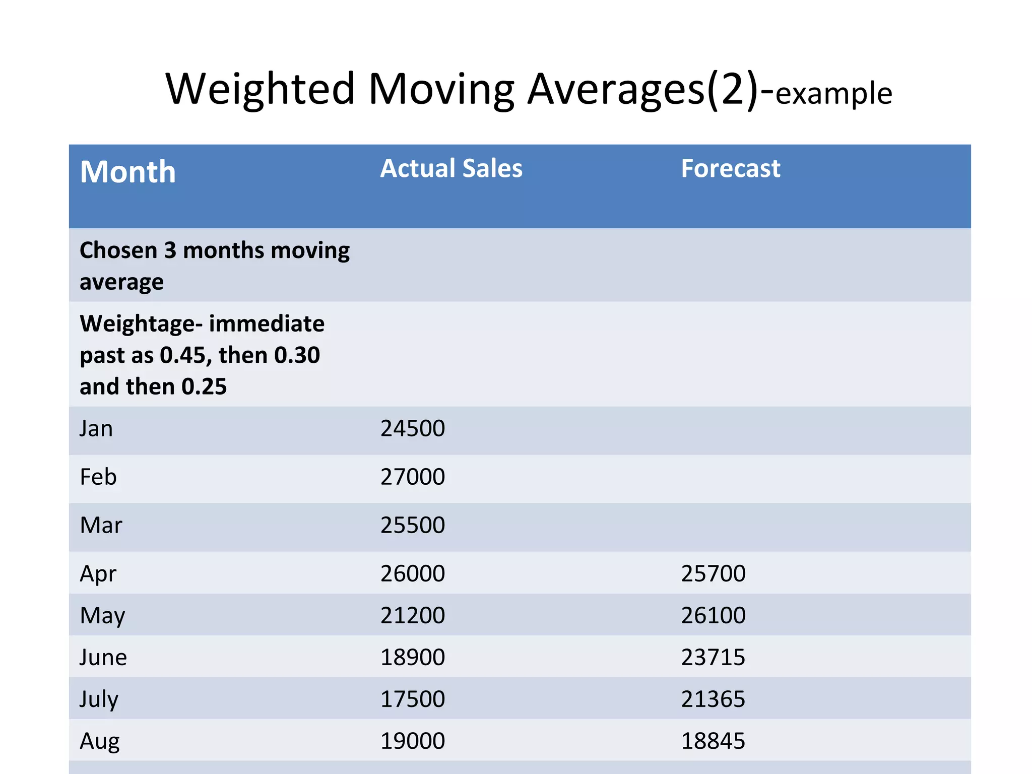
• Assume a mixed model:
Systematic component = (level + trend)(seasonal factor)
Ft+l = [L + (t + l)T]St+l
= forecast in period t for demand in period t + l
L = estimate of level for period 0
T = estimate of trend
St = estimate of seasonal factor for period t
Dt = actual demand in period t
Ft = forecast of demand in period t](https://image.slidesharecdn.com/dpfksraoppt3-131105084513-phpapp02/75/Dpf-ksrao-ppt_3-21-2048.jpg)

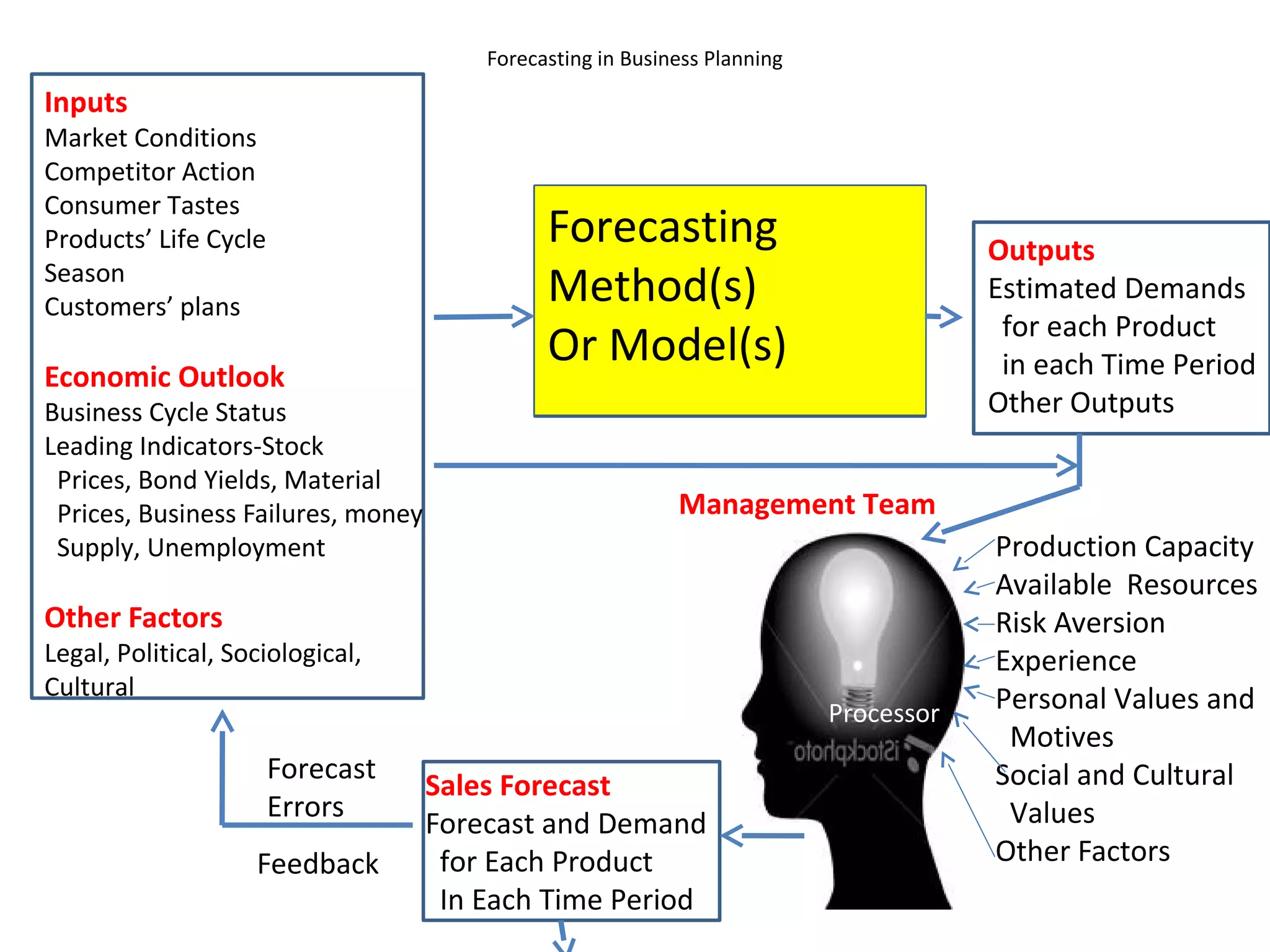
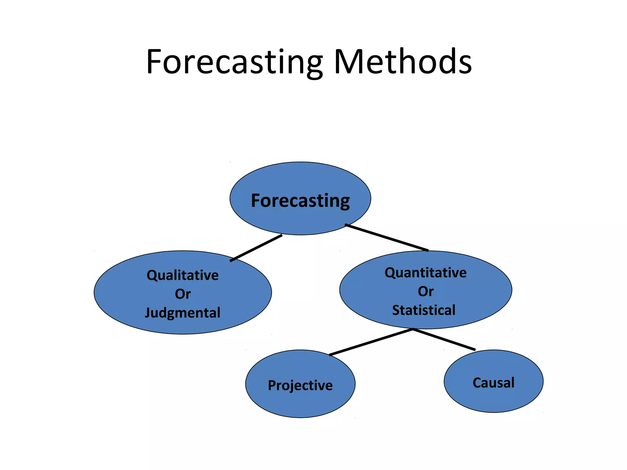
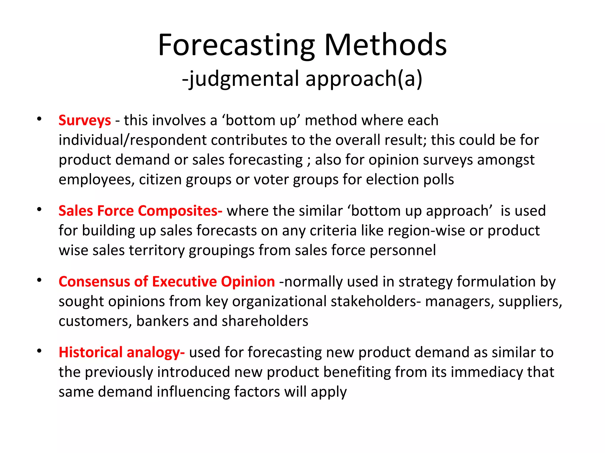
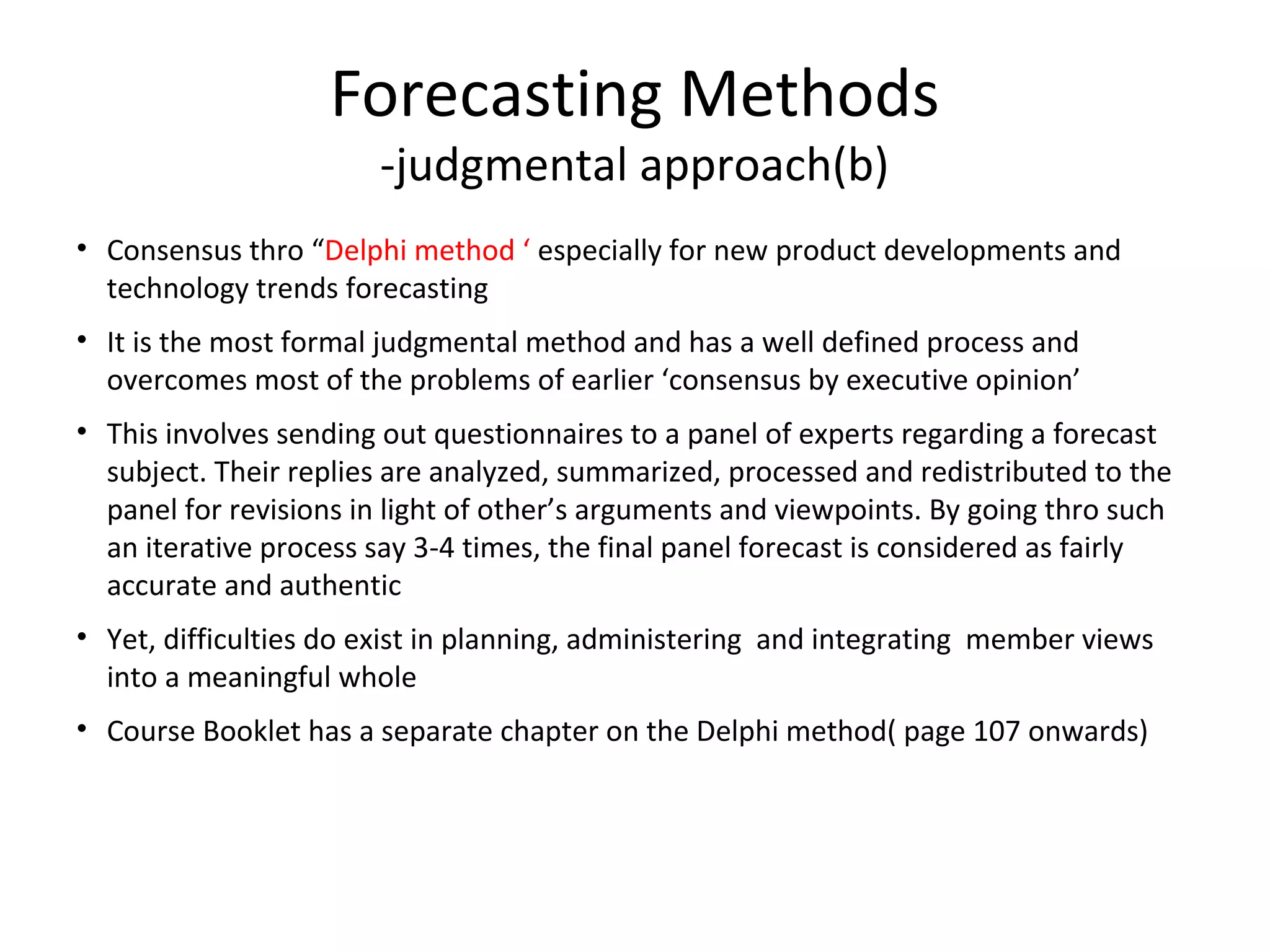
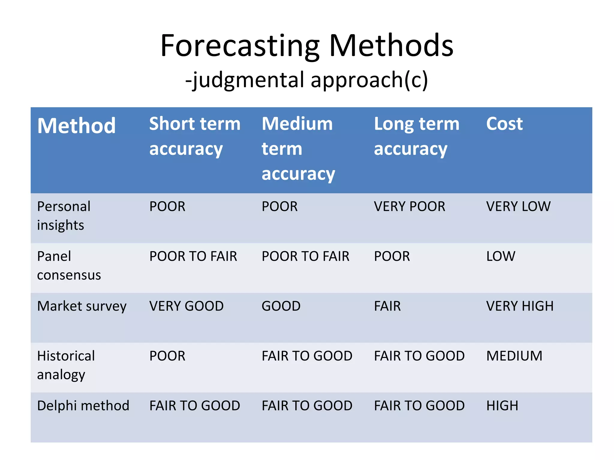
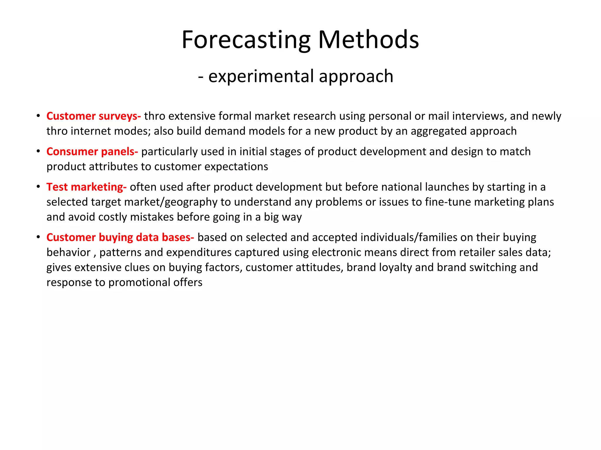
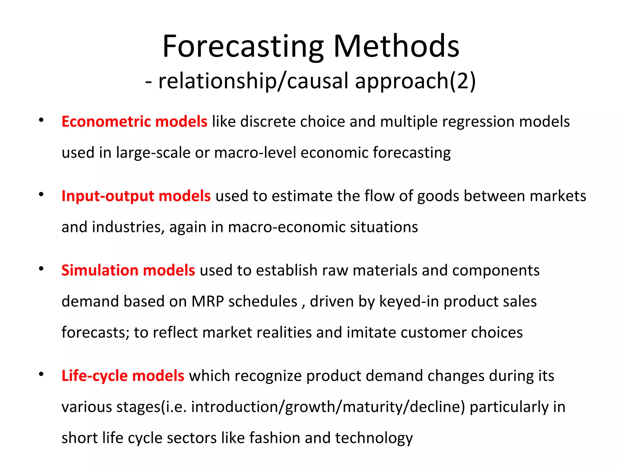
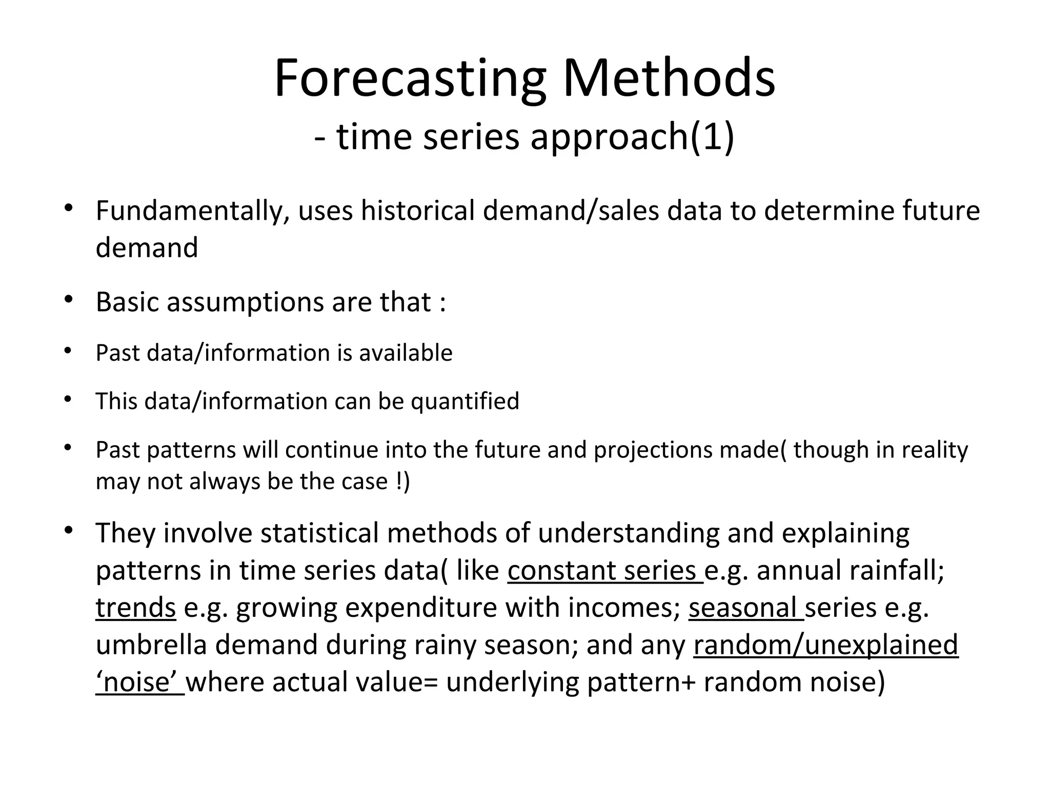
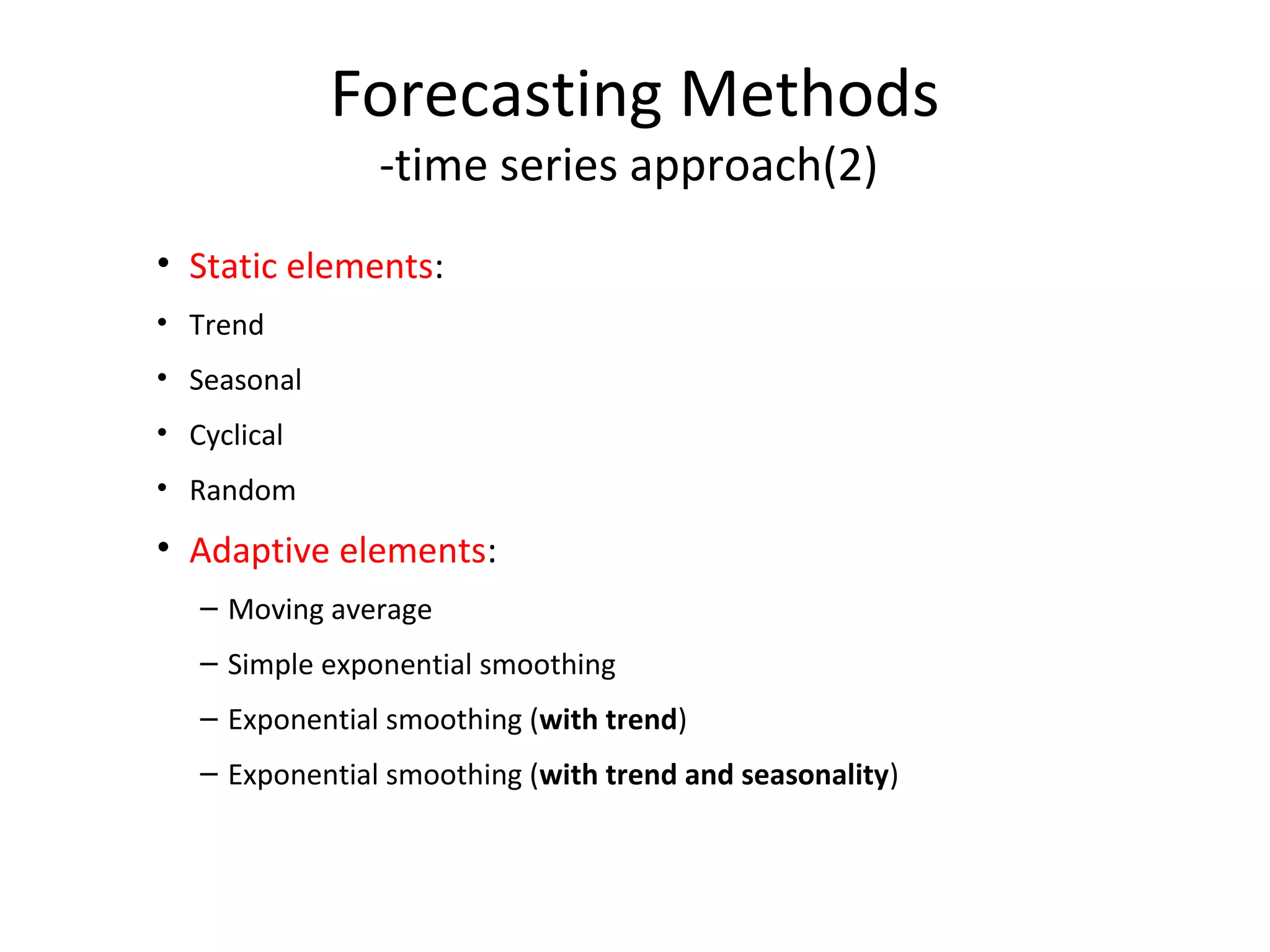
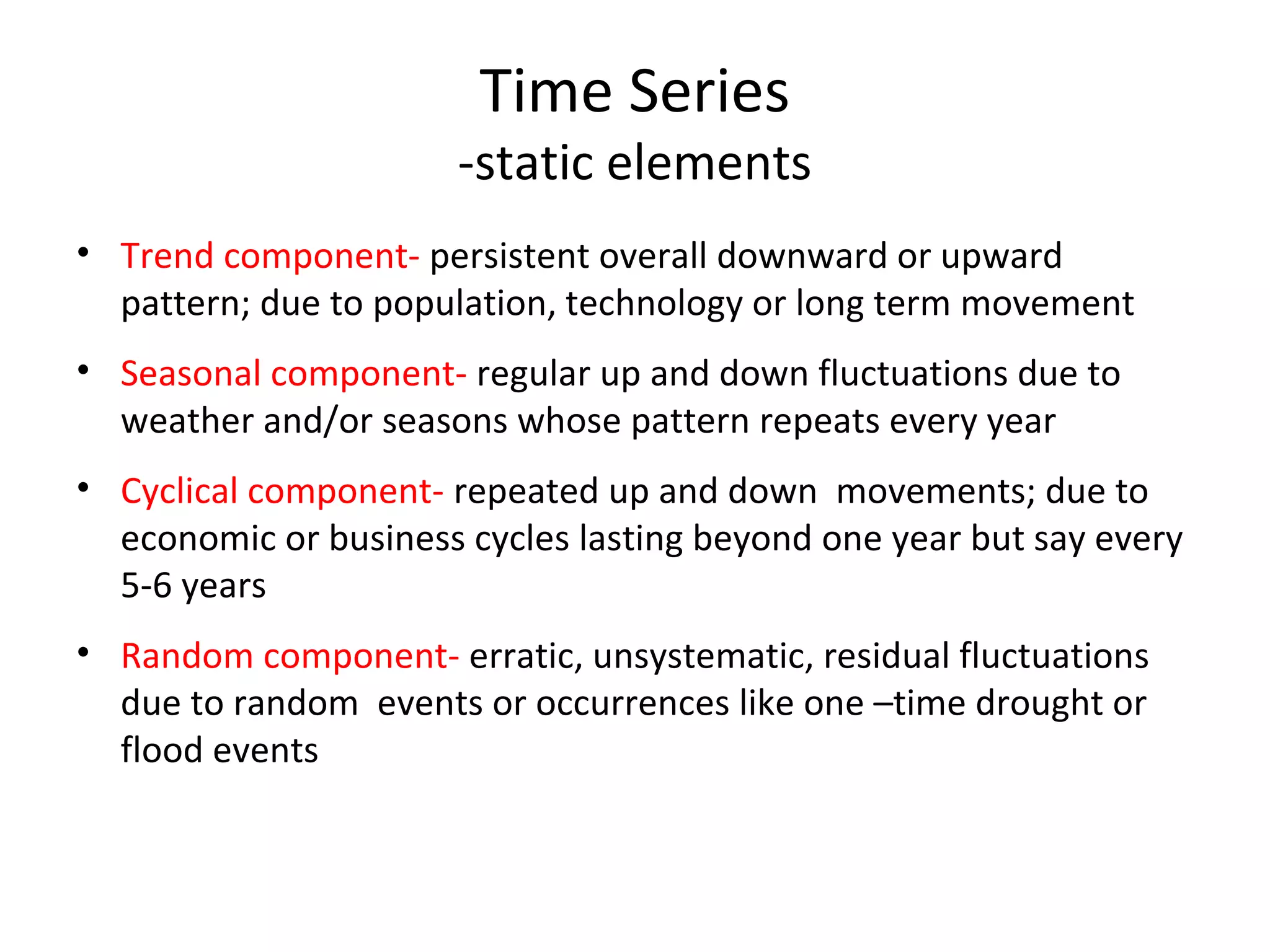
This document discusses various demand forecasting methods. It begins by outlining the inputs and outputs of the forecasting process, as well as factors that influence forecasting like management preferences. It then categorizes forecasting methods as quantitative/statistical or qualitative/judgmental, and as projective or causal. Specific forecasting methods are described in detail, including judgmental approaches like surveys and consensus forecasting. Causal/relationship approaches involving regression models and simulation are also outlined. Finally, time series forecasting is discussed, including different elements like trends and seasons, as well as adaptive methods like moving averages and exponential smoothing.