The document outlines the strategic role of forecasting in supply chain management, detailing various forecasting methods and their components, including time series and regression techniques. It emphasizes the importance of forecast accuracy, the effects of errors, and the need for ongoing monitoring and adjustments in forecasting practices. Additionally, it discusses qualitative and quantitative forecasting approaches alongside practical applications using Excel.

1. Lecture Outline
• Strategic Role of Forecasting in Supply Chain
Management
• Components of Forecasting Demand
• Time Series Methods
• Forecast Accuracy
• Time Series Forecasting Using Excel
• Regression Methods

2. Learning Objectives
• Discuss the strategic role of forecasting in supply
chain management
• Describe the forecasting process and identify the
components of forecasting demand
• Forecast demand using various time series models,
including exponential smoothing, and trend and
seasonal adjustments
• Discuss and calculate various methods for
evaluating forecast accuracy
• Use Excel to create various forecast models
• Develop forecasting models with linear and multiple
regression analysis

3. Forecast
• Forecast – a statement about the future value of
a variable of interest
• We make forecasts about such things as weather,
demand, and resource availability
• Forecasts are important to making informed decisions

4. Two Important Aspects of Forecasts
• Expected level of demand
• The level of demand may be a function of some
structural variation such as trend or seasonal
variation
• Accuracy
• Related to the potential size of forecast error

5. • Plan the system
• Generally involves long-range plans related to:
• Types of products and services to offer
• Facility and equipment levels
• Facility location
• Plan the use of the system
• Generally involves short- and medium-range plans related to:
• Inventory management
• Workforce levels
• Purchasing
• Production
• Budgeting
• Scheduling
Forecast Uses

6. The Effect of Inaccurate Forecasting

7. 1. Techniques assume some underlying causal system
that existed in the past will persist into the future
2. Forecasts are not perfect
3. Forecasts for groups of items are more accurate than
those for individual items
4. Forecast accuracy decreases as the forecasting
horizon increases
Features Common to All Forecasts

8. 3-8
Forecasts are not Perfect
– Forecasts are not perfect:
• Because random variation is always present, there will
always be some residual error, even if all other factors
have been accounted for.

9. The forecast
• should be timely
• should be accurate
• should be reliable
• should be expressed in meaningful units
• should be in writing
• technique should be simple to understand and use
• should be cost-effective
Elements of a Good Forecast

10. 1. Determine the purpose of the forecast
2. Establish a time horizon
3. Obtain, clean, and analyze appropriate data
4. Select a forecasting technique
5. Make the forecast
6. Monitor the forecast errors
Steps in the Forecasting Process

11. 3-
11
Forecast Accuracy and Control
• Allowances should be made for forecast errors
– It is important to provide an indication of the extent to
which the forecast might deviate from the value of the
variable that actually occurs
• Forecast errors should be monitored
– Error = Actual – Forecast
– If errors fall beyond acceptable bounds, corrective
action may be necessary

12. Forecast Accuracy Metrics
n
 
 t
t Forecast
Actual
MAD
 2
t
t
1
Forecast
Actual
MSE




n
n
 


100
Actual
Forecast
Actual
MAPE t
t
t
MAD weights all
errors evenly
MSE weights errors
according to their
squared values
MAPE weights
errors according to
relative error

13. Period
Actual
(A)
Forecast
(F)
(A-F)
Error |Error| Error2 [|Error|/Actual]x100
1 107 110 -3 3 9 2.80%
2 125 121 4 4 16 3.20%
3 115 112 3 3 9 2.61%
4 118 120 -2 2 4 1.69%
5 108 109 1 1 1 0.93%
Sum 13 39 11.23%
n = 5 n-1 = 4 n = 5
MAD MSE MAPE
= 2.6 = 9.75 = 2.25%
Forecast Error Calculation

14. • Qualitative Forecasting
• Qualitative techniques permit the inclusion of soft information
such as:
• Human factors
• Personal opinions
• Hunches
• These factors are difficult, or impossible, to quantify
• Quantitative Forecasting
• These techniques rely on hard data
• Quantitative techniques involve either the projection of historical
data or the development of associative methods that attempt to
use causal variables to make a forecast
• Diffusion Models
Forecasting Approaches

15. 3-
15
Qualitative Forecasts
• Forecasts that use subjective inputs such as opinions from
consumer surveys, sales staff, managers, executives, and experts
– Executive opinions
• a small group of upper-level managers may meet and collectively
develop a forecast
– Sales force opinions
• members of the sales or customer service staff can be good sources of
information due to their direct contact with customers and may be
aware of plans customers may be considering for the future
– Consumer surveys
• since consumers ultimately determine demand, it makes sense to solicit
input from them
• consumer surveys typically represent a sample of consumer opinions
– Other approaches
• managers may solicit 0pinions from other managers or staff people or
outside experts to help with developing a forecast.
• the Delphi method is an iterative process intended to achieve a
consensus

16. 3-
16
Time-Series Forecasts
• Forecasts that project patterns identified in
recent time-series observations
– Time-series - a time-ordered sequence of
observations taken at regular time intervals
• Assume that future values of the time-series can
be estimated from past values of the time-series

17. • Trend
• Seasonality
• Cycles
• Irregular variations
• Random variation
Time-Series Behaviors

18. • Trend
• A long-term upward or downward movement in data
• Population shifts
• Changing income
• Seasonality
• Short-term, fairly regular variations related to the calendar or
time of day
• Restaurants, service call centers, and theaters all experience
seasonal demand
Trends and Seasonality

19. • Cycle
• Wavelike variations lasting more than one year
• These are often related to a variety of economic, political, or even
agricultural conditions
• Irregular variation
• Due to unusual circumstances that do not reflect typical behavior
• Labor strike
• Weather event
• Random Variation
• Residual variation that remains after all other behaviors have
been accounted for
Cycles and Variations

20. Forms of Forecast Movement

21. • Naïve Forecast
• Uses a single previous value of a time series as the
basis for a forecast
• The forecast for a time period is equal to the
previous time period’s value
• Can be used with
• a stable time series
• seasonal variations
• trend
Time-Series Forecasting - Naïve Forecast

22. • These techniques work best when a series tends
to vary about an average
• Averaging techniques smooth variations in the data
• They can handle step changes or gradual changes in
the level of a series
• Techniques
1. Moving average
2. Weighted moving average
3. Exponential smoothing
Time-Series Forecasting - Averaging

23. • Technique that averages a number of the most
recent actual values in generating a forecast
Moving Average
average
moving
in the
periods
of
Number
period
in
value
Actual
average
moving
period
MA
period
for time
Forecast
where
...
MA 1
2
1


















n
i
t
A
n
t
F
n
A
A
A
n
A
F
i
t
n
t
t
t
n
t
n
i
i
t
n
t

24. • As new data become available, the forecast is
updated by adding the newest value and
dropping the oldest and then re-computing the
average
• The number of data points included in the
average determines the model’s sensitivity
• Fewer data points used-- more responsive
• More data points used-- less responsive
Moving Average

25. • The most recent values in a time series are
given more weight in computing a forecast
• The choice of weights, w, is somewhat arbitrary and
involves some trial and error
Weighted Moving Average
etc.
,
1
period
for
value
actual
the
,
period
for
value
actual
the
etc.
,
1
period
for
weight
,
period
for
weight
where
)
(
...
)
(
)
(
1
1
1
1
















t
A
t
A
t
w
t
w
A
w
A
w
A
w
F
t
t
t
t
n
t
n
t
t
t
t
t
t

26. 3-
26
Linear Trend
• A simple data plot can reveal the existence and
nature of a trend
• Linear trend equation
Ft  a  bt
where
Ft  Forecast for period t
a  Value of Ft at t  0
b  Slope of the line
t  Specified number of time periods from t  0

27. • Slope and intercept can be estimated from
historical data
Estimating slope and intercept

b 
n ty  t y



n t2
 t

 

2
a 
y  b t


n
or y  bt
where
n  Number of periods
y  Value of the time series

28. Moving Average: Naïve Approach
Jan 120
Feb 90
Mar 100
Apr 75
May 110
June 50
July 75
Aug 130
Sept 110
Oct 90
ORDERS
MONTH PER MONTH
Nov -
FORECAST

29. Moving Average: Naïve Approach
Jan 120
Feb 90
Mar 100
Apr 75
May 110
June 50
July 75
Aug 130
Sept 110
Oct 90
ORDERS
MONTH PER MONTH
-
120
90
100
75
110
50
75
130
110
90
Nov -
FORECAST

30. Simple Moving Average
MAn =
n
i = 1
 Di
n
where
n = number of periods in
the moving average
Di = demand in period i

31. 3-month Simple Moving Average
Jan 120
Feb 90
Mar 100
Apr 75
May 110
June 50
July 75
Aug 130
Sept 110
Oct 90
Nov -
ORDERS
MONTH PER MONTH
MA3 =
3
i = 1
 Di
3
MOVING
AVERAGE

32. 3-month Simple Moving Average
Jan 120
Feb 90
Mar 100
Apr 75
May 110
June 50
July 75
Aug 130
Sept 110
Oct 90
Nov -
ORDERS
MONTH PER MONTH
MA3 =
3
i = 1
 Di
3
=
90 + 110 + 130
3
= 110 orders for Nov
–
–
–
103.3
88.3
95.0
78.3
78.3
85.0
105.0
110.0
MOVING
AVERAGE

33. 5-month Simple Moving Average
MA5 =
5
i = 1
 Di
5
Jan 120
Feb 90
Mar 100
Apr 75
May 110
June 50
July 75
Aug 130
Sept 110
Oct 90
Nov -
ORDERS
MONTH PER MONTH
MOVING
AVERAGE

34. 5-month Simple Moving Average
MA5 =
5
i = 1
 Di
5
=
90 + 110 + 130+75+50
5
= 91 orders for Nov
Jan 120
Feb 90
Mar 100
Apr 75
May 110
June 50
July 75
Aug 130
Sept 110
Oct 90
Nov -
ORDERS
MONTH PER MONTH
–
–
–
–
–
99.0
85.0
82.0
88.0
95.0
91.0
MOVING
AVERAGE

35. Smoothing Effects

36. Weighted Moving Average
• Adjusts moving average method to more closely
reflect data fluctuations
WMAn =
i = 1
 Wi Di
where
Wi = the weight for period i,
between 0 and 100
percent
 Wi = 1.00
n

37. Weighted Moving Average Example
MONTH WEIGHT DATA
August 17% 130
September 33% 110
October 50% 90
WMA3 =
3
i = 1
 Wi Di
November Forecast

38. Weighted Moving Average Example
MONTH WEIGHT DATA
August 17% 130
September 33% 110
October 50% 90
WMA3 =
3
i = 1
 Wi Di
= (0.50)(90) + (0.33)(110) + (0.17)(130)
= 103.4 orders
November Forecast

39. Exponential Smoothing
• Averaging method
• Weights most recent data more strongly
• Reacts more to recent changes
• Widely used, accurate method
• Smoothing constant, α
• applied to most recent data

40. Exponential Smoothing
Ft +1 = Dt + (1 - )Ft
where:
Ft +1 = forecast for next period
Dt = actual demand for present period
Ft = previously determined forecast for
present period
= weighting factor, smoothing constant

41. 0.0  1.0
If = 0.20, then Ft +1 = 0.20 Dt + 0.80 Ft
If = 0, then Ft +1 = 0 Dt + 1 Ft = Ft
Forecast does not reflect recent data
If = 1, then Ft +1 = 1 Dt + 0 Ft = Dt
Forecast based only on most recent data
Effect of Smoothing Constant

42. Exponential Smoothing (α=0.30)
F2 = D1 + (1 - )F1
F3 = D2 + (1 - )F2
F13 = D12 + (1 - )F12
PERIOD MONTH DEMAND
1 Jan 37
2 Feb 40
3 Mar 41
4 Apr 37
5 May 45
6 Jun 50
7 Jul 43
8 Aug 47
9 Sep 56
10 Oct 52
11 Nov 55
12 Dec 54

43. Exponential Smoothing (α=0.30)
F2 = D1 + (1 - )F1
= (0.30)(37) + (0.70)(37)
= 37
F3 = D2 + (1 - )F2
= (0.30)(40) + (0.70)(37)
= 37.9
F13 = D12 + (1 - )F12
= (0.30)(54) + (0.70)(50.84)
= 51.79
PERIOD MONTH DEMAND
1 Jan 37
2 Feb 40
3 Mar 41
4 Apr 37
5 May 45
6 Jun 50
7 Jul 43
8 Aug 47
9 Sep 56
10 Oct 52
11 Nov 55
12 Dec 54

44. Exponential Smoothing
FORECAST, Ft + 1
PERIOD MONTH DEMAND ( = 0.3) ( = 0.5)
1 Jan 37 – –
2 Feb 40
3 Mar 41
4 Apr 37
5 May 45
6 Jun 50
7 Jul 43
8 Aug 47
9 Sep 56
10 Oct 52
11 Nov 55
12 Dec 54
13 Jan –

45. Exponential Smoothing
FORECAST, Ft + 1
PERIOD MONTH DEMAND ( = 0.3) ( = 0.5)
1 Jan 37 – –
2 Feb 40 37.00 37.00
3 Mar 41 37.90 38.50
4 Apr 37 38.83 39.75
5 May 45 38.28 38.37
6 Jun 50 40.29 41.68
7 Jul 43 43.20 45.84
8 Aug 47 43.14 44.42
9 Sep 56 44.30 45.71
10 Oct 52 47.81 50.85
11 Nov 55 49.06 51.42
12 Dec 54 50.84 53.21
13 Jan – 51.79 53.61

46. Adjusted Exponential Smoothing
AFt +1 = Ft +1 + Tt +1
where
T = an exponentially smoothed trend factor
Tt +1 = (Ft +1 - Ft) + (1 - ) Tt
where
Tt = the last period trend factor
= a smoothing constant for trend
0 ≤  ≤ 1

47. Adjusted Exponential Smoothing (β=0.30)
PERIOD MONTH DEMAND
1 Jan 37
2 Feb 40
3 Mar 41
4 Apr 37
5 May 45
6 Jun 50
7 Jul 43
8 Aug 47
9 Sep 56
10 Oct 52
11 Nov 55
12 Dec 54
T3 = (F3 - F2) + (1 - ) T2
AF3 = F3 + T3
T13 = (F13 - F12) + (1 - ) T12
AF13 = F13 + T13 =

48. Adjusted Exponential Smoothing (β=0.30)
PERIOD MONTH DEMAND
1 Jan 37
2 Feb 40
3 Mar 41
4 Apr 37
5 May 45
6 Jun 50
7 Jul 43
8 Aug 47
9 Sep 56
10 Oct 52
11 Nov 55
12 Dec 54
T3 = (F3 - F2) + (1 - ) T2
= (0.30)(38.5 - 37.0) + (0.70)(0)
= 0.45
AF3 = F3 + T3 = 38.5 + 0.45
= 38.95
T13 = (F13 - F12) + (1 - ) T12
= (0.30)(53.61 - 53.21) + (0.70)(1.77)
= 1.36
AF13 = F13 + T13 = 53.61 + 1.36 = 54.97

49. Adjusted Exponential Smoothing
FORECAST TREND ADJUSTED
PERIOD MONTH DEMAND Ft +1 Tt +1 FORECAST AFt +1
1 Jan 37 37.00 – –
2 Feb 40 37.00 0.00 37.00
3 Mar 41 38.50 0.45 38.95
4 Apr 37 39.75 0.69 40.44
5 May 45 38.37 0.07 38.44
6 Jun 50 38.37 0.07 38.44
7 Jul 43 45.84 1.97 47.82
8 Aug 47 44.42 0.95 45.37
9 Sep 56 45.71 1.05 46.76
10 Oct 52 50.85 2.28 58.13
11 Nov 55 51.42 1.76 53.19
12 Dec 54 53.21 1.77 54.98
13 Jan – 53.61 1.36 54.96

50. Adjusted Exponential Smoothing
FORECAST TREND ADJUSTED
PERIOD MONTH DEMAND Ft +1 Tt +1 FORECAST AFt +1
1 Jan 37
2 Feb 40
3 Mar 41
4 Apr 37
5 May 45
6 Jun 50
7 Jul 43
8 Aug 47
9 Sep 56
10 Oct 52
11 Nov 55
12 Dec 54
13 Jan –

51. • Seasonality – regularly repeating movements in
series values that can be tied to recurring events
• Expressed in terms of the amount that actual values
deviate from the average value of a series
• Models of seasonality
• Additive
• Seasonality is expressed as a quantity that gets added to
or subtracted from the time-series average in order to
incorporate seasonality
• Multiplicative
• Seasonality is expressed as a percentage of the average
(or trend) amount which is then used to multiply the value
of a series in order to incorporate seasonality
Techniques for Seasonality

52. • Seasonal relatives
• The seasonal percentage used in the multiplicative seasonally
adjusted forecasting model
• Using seasonal relatives
• To deseasonalize data
• Done in order to get a clearer picture of the nonseasonal
(e.g., trend) components of the data series
• Divide each data point by its seasonal relative
• To incorporate seasonality in a forecast
1. Obtain trend estimates for desired periods using a trend
equation
2. Add seasonality by multiplying these trend estimates by the
corresponding seasonal relative
Seasonal Relatives

53. Seasonal Adjustments
 Repetitive increase/ decrease in demand
 Use seasonal factor to adjust forecast
Seasonal factor = Si =
Di
D

54. Seasonal Adjustment
2002 12.6 8.6 6.3 17.5
2003 14.1 10.3 7.5 18.2
2004 15.3 10.6 8.1 19.6
DEMAND (1000’S PER QUARTER)
YEAR 1 2 3 4 Total
S1 = =
D1
D
S2 = =
D2
D
S4 = =
D4
D
S3 = =
D3
D

55. Seasonal Adjustment
SF1 = (S1) (F5) =
SF2 = (S2) (F5) =
SF3 = (S3) (F5) =
SF4 = (S4) (F5) =
y =
For 2005

56. Seasonal Adjustment
2002 12.6 8.6 6.3 17.5 45.0
2003 14.1 10.3 7.5 18.2 50.1
2004 15.3 10.6 8.1 19.6 53.6
Total 42.0 29.5 21.9 55.3 148.7
DEMAND (1000’S PER QUARTER)
YEAR 1 2 3 4 Total
S1 = = = 0.28
D1
D
42.0
148.7
S2 = = = 0.20
D2
D
29.5
148.7
S4 = = = 0.37
D4
D
55.3
148.7
S3 = = = 0.15
D3
D
21.9
148.7

57. Seasonal Adjustment
SF1 = (S1) (F5) = (0.28)(58.17) = 16.28
SF2 = (S2) (F5) = (0.20)(58.17) = 11.63
SF3 = (S3) (F5) = (0.15)(58.17) = 8.73
SF4 = (S4) (F5) = (0.37)(58.17) = 21.53
y = 40.97 + 4.30x = 40.97 + 4.30(4) = 58.17
For 2005

58. • Associative techniques are based on the
development of an equation that summarizes
the effects of predictor variables
• Predictor variables - variables that can be used to
predict values of the variable of interest
• Home values may be related to such factors as
home and property size, location, number of
bedrooms, and number of bathrooms
Associative Forecasting Techniques

59. • Regression - a technique for fitting a line to a set
of data points
• Simple linear regression - the simplest form of
regression that involves a linear relationship between
two variables
• The object of simple linear regression is to obtain
an equation of a straight line that minimizes the
sum of squared vertical deviations from the line
(i.e., the least squares criterion)
Simple Linear Regression

60. Least Squares Line
    
   
ns
observatio
paired
of
Number
where
or
and
intercept)
at the
line
the
of
height
the
(i.e.,
0
when
of
Value
line
the
of
Slope
variable
nt)
(independe
Predictor
variable
)
(dependent
Predicted
where
2
2














 





n
x
b
y
n
x
b
y
a
x
x
n
y
x
xy
n
b
y
x
y
a
b
x
y
bx
a
y
c
c
c

61. • Correlation, r
• A measure of the strength and direction of relationship between
two variables
• Ranges between -1.00 and +1.00
• r2, square of the correlation coefficient
• A measure of the percentage of variability in the values of y that
is “explained” by the independent variable
• Ranges between 0 and 1.00
Correlation Coefficient
    
       2
2
2
2











y
y
n
x
x
n
y
x
xy
n
r

62. Linear Regression Example
x y
(WINS) (ATTENDANCE) xy x2
4 36.3 145.2 16
6 40.1 240.6 36
6 41.2 247.2 36
8 53.0 424.0 64
6 44.0 264.0 36
7 45.6 319.2 49
5 39.0 195.0 25
7 47.5 332.5 49
49 346.7 2167.7 311

63. Linear Regression Example
x = = 6.125
y = = 43.36
b =
=
= 4.06
a = y - bx
= 43.36 - (4.06)(6.125)
= 18.46
49
8
346.9
8
xy - nxy2
x2 - nx2
(2,167.7) - (8)(6.125)(43.36)
(311) - (8)(6.125)2

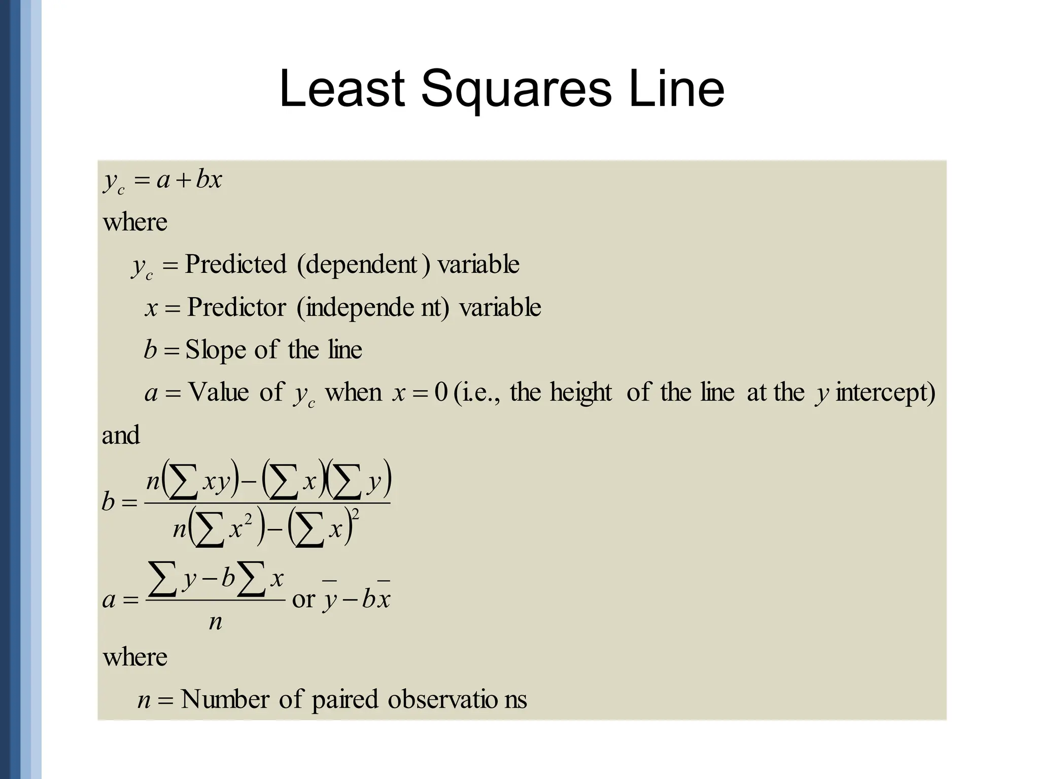
64. n xy -  x y
[n x2 - ( x)2] [n y2 - ( y)2]
r =
Computing Correlation

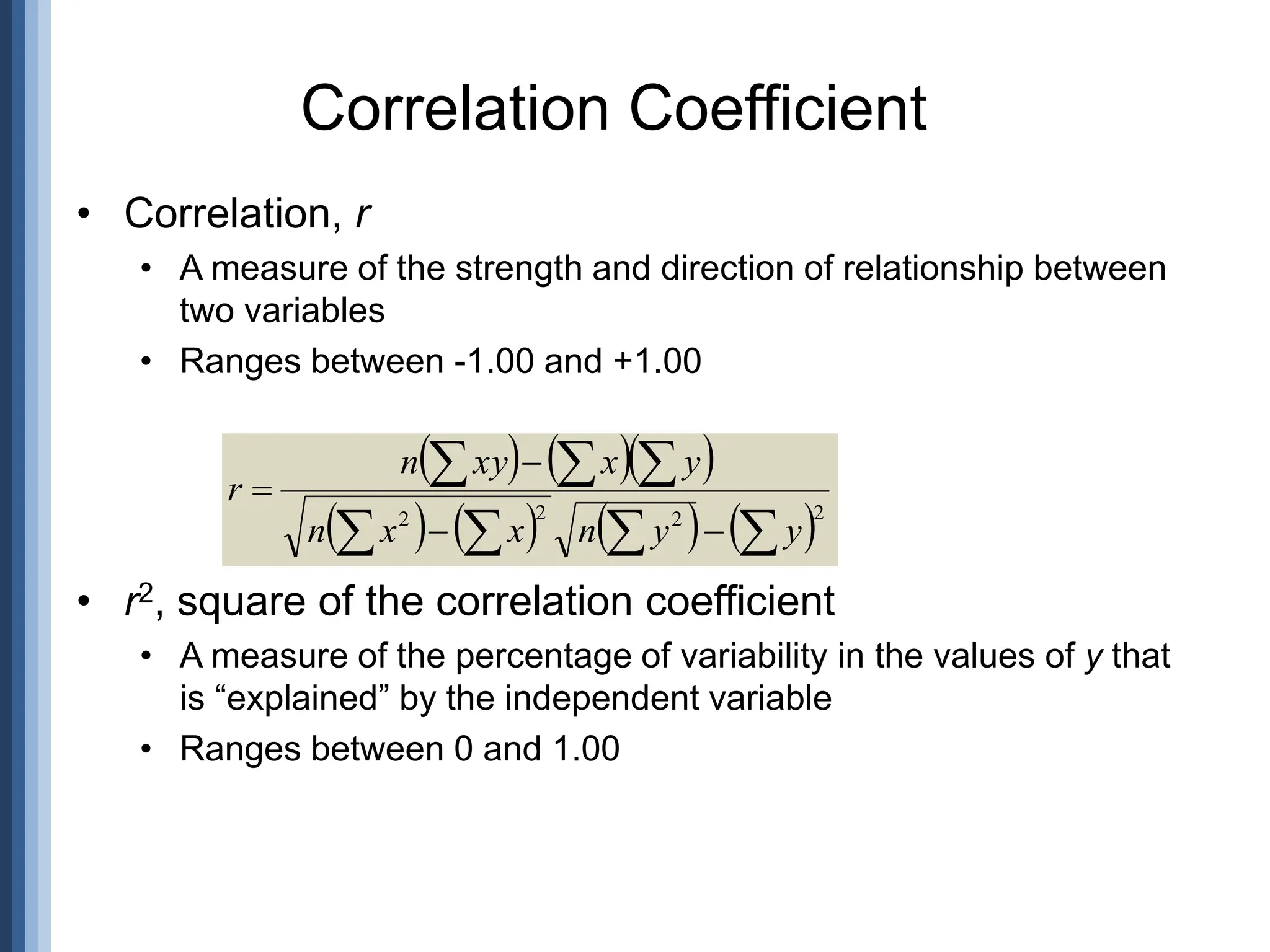
65. n xy -  x y
[n x2 - ( x)2] [n y2 - ( y)2]
r =
Coefficient of determination
r2 = (0.947)2 = 0.897
r =
(8)(2,167.7) - (49)(346.9)
[(8)(311) - (49)2] [(8)(15,224.7) - (346.9)2]
r = 0.947
Computing Correlation

66. 3-
68
Simple Linear Regression Assumptions
1. Variations around the line are random
2. Deviations around the average value (the line)
should be normally distributed
3. Predictions are made only within the range of
observed values

67. • Always plot the line to verify that a linear
relationship is appropriate
• The data may be time-dependent.
• If they are
• use analysis of time series
• use time as an independent variable in a multiple
regression analysis
• A small correlation may indicate that other
variables are important
Issues to consider:

68. • Tracking forecast errors and analyzing them can provide
useful insight into whether forecasts are performing
satisfactorily
• Sources of forecast errors:
• The model may be inadequate due to
a. omission of an important variable
b. a change or shift in the variable the model cannot handle
c. the appearance of a new variable
• Irregular variations may have occurred
• Random variation
• Control charts are useful for identifying the presence of non-
random error in forecasts
• Tracking signals can be used to detect forecast bias
Monitoring the Forecast

69. Forecast Control
• Tracking signal
• monitors the forecast to see if it is biased high or low
• 1 MAD ≈ 0.8𝜎 Control limits of 2 to 5 MADs are used
most frequently
Tracking signal = =
(Dt - Ft)
MAD
E
MAD

70. Tracking Signal Values
1 37 37.00 – – –
2 40 37.00 3.00 3.00 3.00
3 41 37.90 3.10 6.10 3.05
4 37 38.83 -1.83 4.27 2.64
5 45 38.28 6.72 10.99 3.66
6 50 40.29 9.69 20.68 4.87
7 43 43.20 -0.20 20.48 4.09
8 47 43.14 3.86 24.34 4.06
9 56 44.30 11.70 36.04 5.01
10 52 47.81 4.19 40.23 4.92
11 55 49.06 5.94 46.17 5.02
12 54 50.84 3.15 49.32 4.85
DEMAND FORECAST, ERROR E =
PERIOD Dt Ft Dt - Ft (Dt - Ft) MAD

71. Tracking Signal Values
1 37 37.00 – – –
2 40 37.00 3.00 3.00 3.00
3 41 37.90 3.10 6.10 3.05
4 37 38.83 -1.83 4.27 2.64
5 45 38.28 6.72 10.99 3.66
6 50 40.29 9.69 20.68 4.87
7 43 43.20 -0.20 20.48 4.09
8 47 43.14 3.86 24.34 4.06
9 56 44.30 11.70 36.04 5.01
10 52 47.81 4.19 40.23 4.92
11 55 49.06 5.94 46.17 5.02
12 54 50.84 3.15 49.32 4.85
DEMAND FORECAST, ERROR E =
PERIOD Dt Ft Dt - Ft (Dt - Ft) MAD
–
1.00
2.00
1.62
3.00
4.25
5.01
6.00
7.19
8.18
9.20
10.17
TRACKING
SIGNAL
TS3 = = 2.00
6.10
3.05

72. Tracking Signal Plot

73. Statistical Control Charts
 =
(Dt - Ft)2
n - 1
 Using  we can calculate statistical control limits
for the forecast error
 Control limits are typically set at  3
Mean squared error (MSE)
Average of squared forecast errors

74. Statistical Control Charts

75. 77
S-curve of Technology Diffusion
Decline
Saturation
Learning
Time
Growth
Current
Technology
Emerging
Technology
Growth

76. 78
Technology Diffusion
• Technology diffusion is typically modelled as an S-shaped
curve over time
• Assumption is that there is an upper limit to the growth of a
technology
• Growth pattern follows a logistic path
• Each technology undergoes four different phases: learning,
growth, saturation, and decline

77. 79
Two distributions of f(x) with
thresholds separating adopters from
non-adopters
Source; Geroky, 2000
https://doi.org/10.1016/S0048-7333(99)00092-X
x = Characteristic determining the
profitability of adopting a
technology.

78. 80
Rate of adoption of the innovation

79. 81
Position of individual SET relative to market
penetration
Technology maturity
by stage
Market
Penetration
(indicative)
Research
Demonstration
Pre-
commercial
Support
commercial
Fully
commercial
1. Solar water
heating
1
2
2. Solar cooker
3
3. Solar electricity
4
4. Solar PV
5
5. Wind Energy
6
6. Small hydro
7
7. Biomass/
Cogeneration
8
8. Energy to waste
9. Hydrogen/ Fuel-
cell/ BOV/ Bio fuels
9
10. Geothermal/
Tidal
10

80. 82

81. 3-
83
Choosing a Forecasting Technique
• Factors to consider
– Cost
– Accuracy
– Availability of historical data
– Availability of forecasting software
– Time needed to gather and analyze data and prepare
a forecast
– Forecast horizon

82. • The better forecasts are, the more able organizations will
be to take advantage of future opportunities and reduce
potential risks
• A worthwhile strategy is to work to improve short-term forecasts
• Accurate up-to-date information can have a significant effect
on forecast accuracy:
• Prices
• Demand
• Other important variables
• Reduce the time horizon forecasts have to cover
• Sharing forecasts or demand data through the
supply chain can improve forecast quality
Operations Strategy