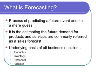
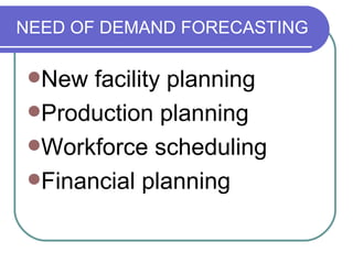
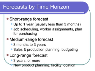
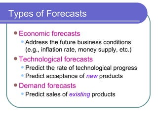
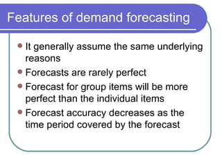
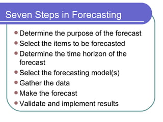
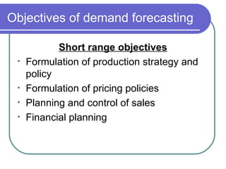
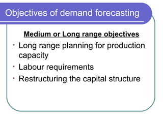
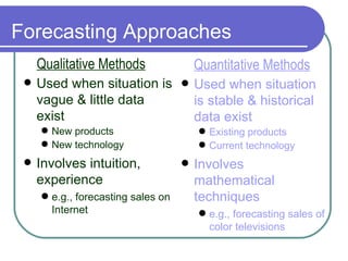
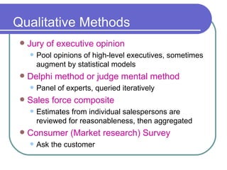
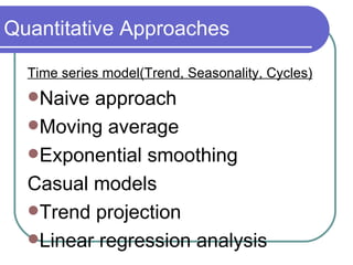
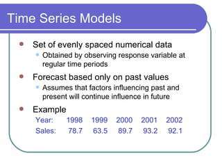
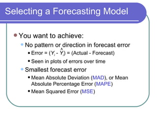
Forecasting involves predicting future events and is commonly used to estimate future demand for products and services. There are different time horizons for forecasts, including short-range (up to 1 year), medium-range (3 months to 3 years), and long-range (3 years or more). Forecasting methods can be quantitative, using mathematical techniques and historical data, or qualitative, using intuition and expert opinions. The objectives of demand forecasting include production planning, financial planning, and long-term strategic planning.

1. Forecasting

2. What is Forecasting? Process of predicting a future event and it is a mere guess. It is the estimating the future demand for products and services are commonly referred as a sales forecast Underlying basis of all business decisions: Production Inventory Personnel Facilities

3. NEED OF DEMAND FORECASTING New facility planning Production planning Workforce scheduling Financial planning

4. Short-range forecast Up to 1 year (usually less than 3 months) Job scheduling, worker assignments, plan for purchasing Medium-range forecast 3 months to 3 years Sales & production planning, budgeting Long-range forecast 3 years, or more New product planning, facility location Forecasts by Time Horizon

5. Types of Forecasts Economic forecasts Address the future business conditions (e.g., inflation rate, money supply, etc.) Technological forecasts Predict the rate of technological progress Predict acceptance of new products Demand forecasts Predict sales of existing products

6. Features of demand forecasting It generally assume the same underlying reasons Forecasts are rarely perfect Forecast for group items will be more perfect than the individual items Forecast accuracy decreases as the time period covered by the forecast

7. Seven Steps in Forecasting Determine the purpose of the forecast Select the items to be forecasted Determine the time horizon of the forecast Select the forecasting model(s) Gather the data Make the forecast Validate and implement results

8. Objectives of demand forecasting Short range objectives Formulation of production strategy and policy Formulation of pricing policies Planning and control of sales Financial planning

9. Objectives of demand forecasting Medium or Long range objectives Long range planning for production capacity Labour requirements Restructuring the capital structure

10. Forecasting Approaches Used when situation is stable & historical data exist Existing products Current technology Involves mathematical techniques e.g., forecasting sales of color televisions Quantitative Methods Used when situation is vague & little data exist New products New technology Involves intuition, experience e.g., forecasting sales on Internet Qualitative Methods

11. Qualitative Methods Jury of executive opinion Pool opinions of high-level executives, sometimes augment by statistical models Delphi method or judge mental method Panel of experts, queried iteratively Sales force composite Estimates from individual salespersons are reviewed for reasonableness, then aggregated Consumer (Market research) Survey Ask the customer

12. Quantitative Approaches Time series model(Trend, Seasonality, Cycles) Naive approach Moving average Exponential smoothing Casual models Trend projection Linear regression analysis

13. Set of evenly spaced numerical data Obtained by observing response variable at regular time periods Forecast based only on past values Assumes that factors influencing past and present will continue influence in future Example Year: 1998 1999 2000 2001 2002 Sales: 78.7 63.5 89.7 93.2 92.1 Time Series Models

14. Time Series Components Trend Seasonal Cycle Random

15. Persistent, overall upward or downward pattern Due to population, technology etc. Several years duration Trend Component

16. Regular pattern of up & down fluctuations Due to weather, customs, etc. Occurs within 1 year Seasonal Component

17. Repeating up & down movements Due to interactions of factors influencing economy Can be anywhere between 2-30+ years duration Cyclical Component

18. Erratic, unsystematic, ‘residual’ fluctuations Due to random variation or unforeseen events Union strike Tornado Short duration & non-repeating Random Component

19. 1.Naive Approach Assumes demand in next period is equal to the actual demand in most recent period e.g., If May sales were 48, then June sales will be 48 Sometimes cost effective & efficient

20. Moving average uses a number of most recent historical actual data values to generate a forecast. MA is a series of arithmetic means Used if little or no trend Used often for smoothing Provides overall impression of data over time Equation: 2.Moving Average Method MA n n   Demand in Previous Periods

21. example Forecast demand for 4 months d1+d2+d3 *4 3

22. 3.Exponential Smoothing Method It requires only three items of data this periods forecast, the actual demand for this period and α which is referred to as a smoothing constant and having value between 0 and 1 Next period’s forecast = This period forecast + α { this period’s actual dd – this periods forecast}

23. F t = F t -1 +  ( A t -1 - F t -1 ) F t = forecast for this period F t -1 = forecast for the previous period A t -1= Actual demand for the previous period  Smoothing constant (0 to 1) Exponential Smoothing Equations

24. Used for forecasting linear trend line Assumes relationship between response variable, Y, and time, X, is a linear function Estimated by least squares method Minimizes sum of squared errors Linear Trend Projection i Y a bX i  

25. Answers: ‘ how strong is the linear relationship between the variables?’ Coefficient of correlation Sample correlation coefficient denoted r Range: -1 < r < 1 Measures degree of association Used mainly for understanding Correlation

26. Linear regression analysis The demand or sales forecast is a dependent variable and other factors are independent variables

27. Factors to be considered in the selection of forecasting method Cost and accuracy Data available Time span Nature of products and services Impulse response and noise dampening

28. You want to achieve: No pattern or direction in forecast error Error = ( Y i - Y i ) = (Actual - Forecast) Seen in plots of errors over time Smallest forecast error Mean Absolute Deviation ( MAD ), or Mean Absolute Percentage Error ( MAPE ) Mean Squared Error ( MSE ) Selecting a Forecasting Model ^

29. Which Model Is “Best” So Far? The Naïve model has both the lowest MAD (1.91) and MSE (4.45) of the first five models tested Therefore, the Naïve model is the “best” However, it may be that one model has the lowest MAD or MAPE and another model has the lowest MSE …

30. So Which Model Do You Choose? If you only require the forecast with the smallest average deviation, choose the model with the smallest MAD or MAPE However, if you have a low tolerance for large deviations choose the model with the smallest MSE