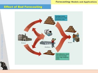
This document provides an overview of operations management forecasting models and their applications. It defines forecasting and lists its common uses. The key components of a forecast and the forecasting process are described. Both qualitative and quantitative forecasting approaches are discussed, along with their advantages and disadvantages. Specific forecasting techniques covered include time series methods, regression methods, moving averages, exponential smoothing, and naive forecasts. Examples are provided to illustrate weighted moving averages and exponential smoothing.


![OperationsManagement
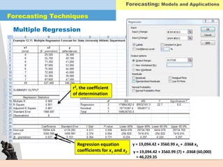
Correlation, r
• Measure of strength of relationship
• Varies between -1.00 and +1.00
Coefficient of determination, r2
• Percentage of variation in dependent variable resulting
from changes in the independent variable
Computing coefficient of correlation:
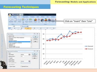
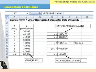
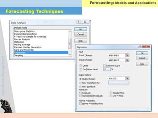
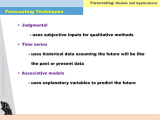
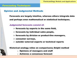
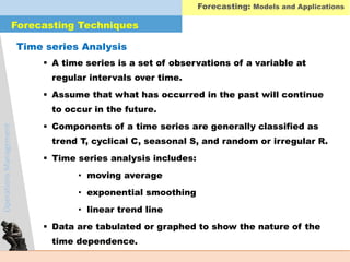
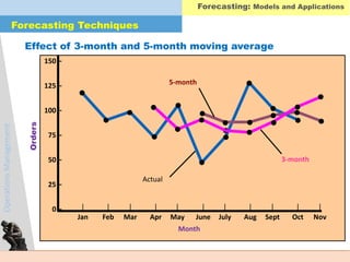
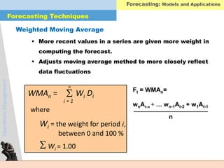
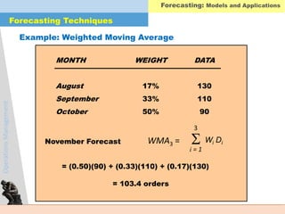
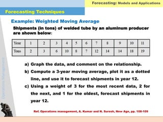
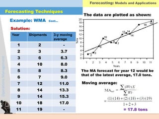
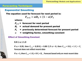
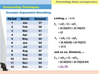
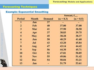
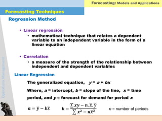
Forecasting Techniques
Forecasting: Models and Applications
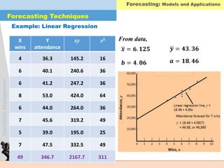
Correlation
n xy - x y
[n x2 - ( x)2] [n y2 - ( y)2]
r =
(8)(2,167.7) - (49)(346.9)
[(8)(311) - (49)2] [(8)(15,224.7) - (346.9)2]
r = =0.947](https://image.slidesharecdn.com/enggmanagementforecasting-190818015810/85/Forecasting-Models-Their-Applications-38-320.jpg)