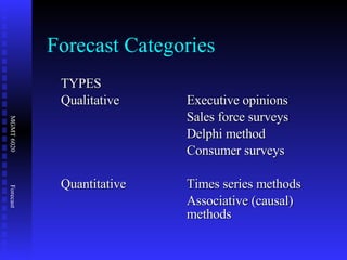
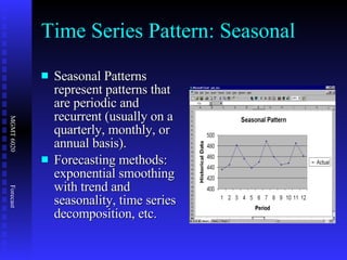
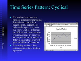
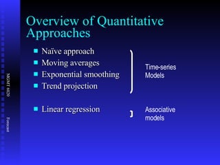
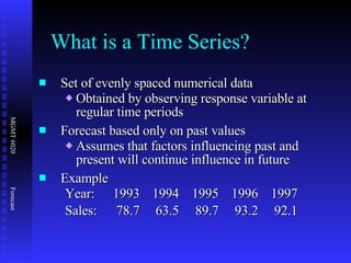
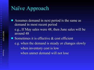
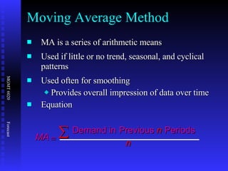
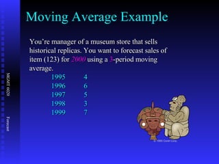
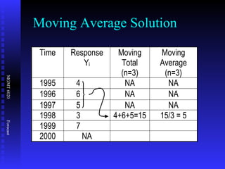
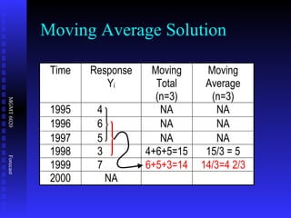
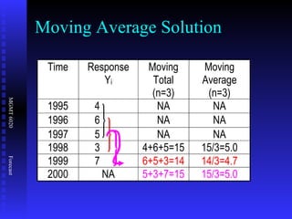
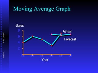
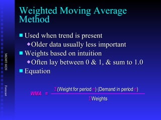
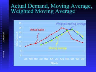
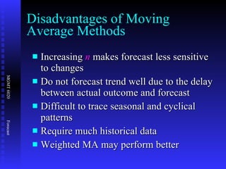
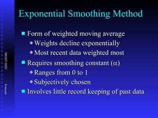
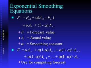
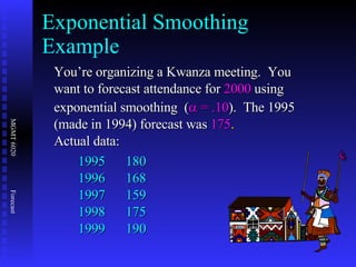
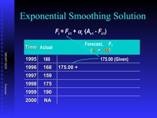
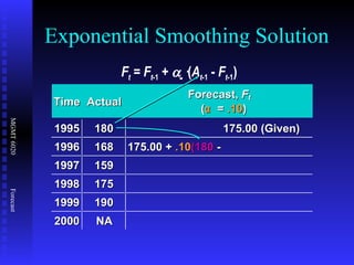
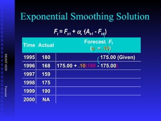
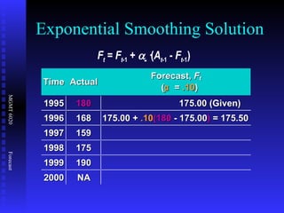
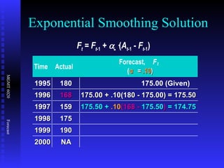
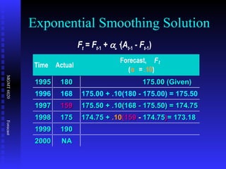
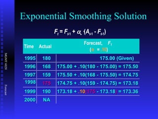
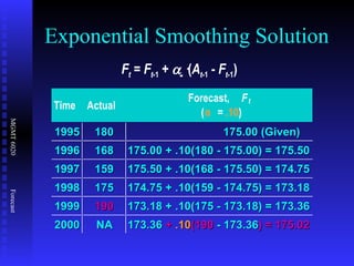
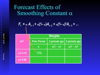
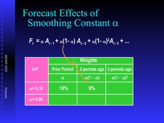
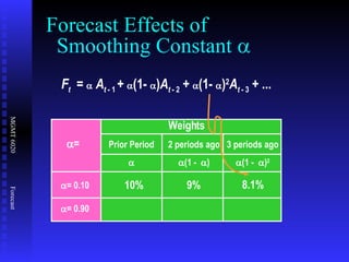
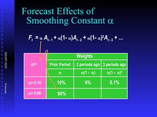
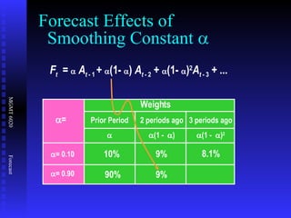
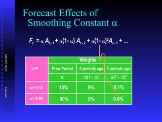
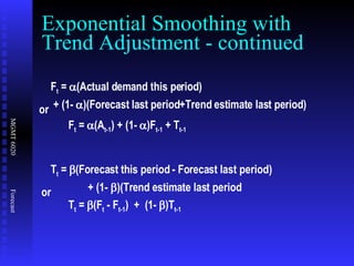
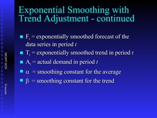
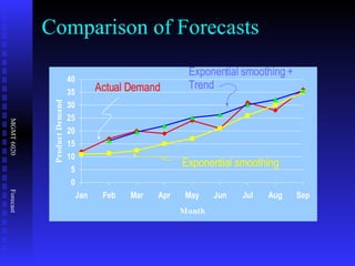
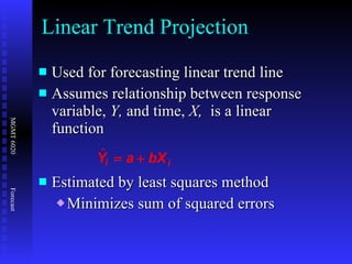
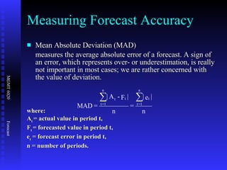
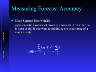
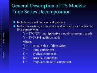
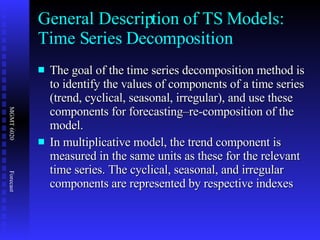
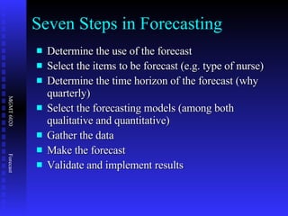
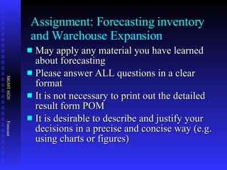
The document discusses various quantitative forecasting techniques including time series methods like moving averages and exponential smoothing. It provides examples of how to calculate 3-period moving averages and exponential smoothing forecasts using sample sales data. Exponential smoothing places more weight on recent observations compared to moving averages. The smoothing constant determines how quickly older data is discounted.

1. Forecasting Outlines Forecasting in Operations Management Science and Art of Forecasting Seven Steps in the Forecasting Categories and Models of Forecasting (Focus on Time-Series Forecasting) Measure the Forecast Accuracy Selecting the Best Forecasting Techniques Forecasting in service sector; forecasting and IT

2. Learning Objectives When you complete this chapter, you should be able to : Identify or Define : Forecasting Categories of forecasts Time horizons Approaches to measure forecasts Explain and Apply: Moving averages Exponential smoothing Trend and seasonal projections Measures of forecast accuracy

3. Why Forecasting? Forecasting lays a ground for reducing the risk in all decision making because many of the decisions need to be made under uncertainty. In business applications, forecasting serves as a starting point of major decisions in finance, marketing, productions, and purchasing. Under what condition there is no value for forecasting?

4. Decisions Requiring Forecasting in Operations Management Predicting demands of new and existing products Predicting results of new product research and development Projecting quality improvement Anticipating customer’s needs Predicting cost of materials

5. Decisions Relevant to Demand Forecasts Select product portfolio Predicting new facility location Anticipating capacity needs Identifying labor requirements Projecting material requirements Developing production schedules Creating maintenance schedules

6. Forecasting at Tupperware Via forecasting, managers make important decisions Each of 50 profit centers around the world is responsible for computerized monthly, quarterly, and 12-month sales projections These projections are aggregated by product family and region, then globally, at Tupperware’s World Headquarters Tupperware uses all techniques discussed in text

7. Successful Forecasting = Science + Art "Science" implies that the body of the forecasting knowledge lies on the solid ground of quantitative forecasting methods and their correct utilization for various business situations. "Art" represents a combination of a decision maker's experience, logic, and intuition to supplement the forecasting quantitative analysis. Both the science and art of forecasting are essential in developing accurate forecasts. All managers are forecasters!

8. Forecast Categories TYPES Qualitative Executive opinions Sales force surveys Delphi method Consumer surveys Quantitative Times series methods Associative (causal) methods

9. For Tupperware’s Strategic Decisions - Forecast by Consensus Although inputs come from sales, marketing, finance, and production, final forecasts are the consensus of all participating managers. The final step is Tupperware’s version of the “jury of executive opinion” Use quantitative models to examine data and use qualitative methods to converge results

10. Forecast Categories TIME HORIZON Long-term For duration of 3-5 years or more (on annual basis) Medium-term For duration of up to three years (usually on quarterly or monthly basis) Short-term Up to one year, usually less than three months (on daily, weekly)

11. Facts in Forecasting Main assumption: Past pattern repeats itself into the future. Forecasts are rarely perfect: Don't expect forecasts to be exactly equal to the actual data. The science and art of forecasting try to minimize, but not to eliminate, forecast errors. Forecast errors mean the difference between actual and forecasted values. Forecasts for a group of products are usually more accurate than these for individual products; a shorter period tend to be more accurate. Computer and IT are critical parts of the modern forecasting in large corporations.

12. Seven Steps in Forecasting (Demands) Determine the use of the forecast Select the items to be forecast Determine the time horizon of the forecast Select the forecasting model(s) Gather the data Make the forecast Validate and implement results

13. Quantitative Methods A time series is an uninterrupted set of data observations that have been ordered in equally spaced intervals (units of time). Associative (causal) forecasting is based on identification of variables (factors) that can predict values of the variable in question.

14. Quantitative Forecasting Models · Time Series Models Naive Forecast Simple Moving Averages Weighted Moving Averages Simple Exponential Smoothing Exponential Smoothing with Trend Linear Trend Projection Time Series Decomposition · Associative (Causal) Models Simple Linear Regression Multiple Linear Regression Nonlinear Regression

15. Time Series Pattern: Stationary The result of many influences that act independently so as to yield nonsystematic and non-repeating patterns about some average value. Forecasting methods: naive, moving average, exponential smoothing

16. Time Series Pattern: Trend It represents a general increase or decrease in a time series over several consecutive periods (some sources present six-seven or more periods). Forecasting methods: linear trend projection, exponential smoothing with trend, etc.

17. Time Series Pattern: Seasonal Seasonal Patterns represent patterns that are periodic and recurrent (usually on a quarterly, monthly, or annual basis). Forecasting methods: exponential smoothing with trend and seasonality, time series decomposition, etc.

18. Time Series Pattern: Cyclical The result of economic and business expansions (increasing demand) and contractions (recessions and depressions) and usually repeat every two-five years. Cyclical influences are difficult to forecast because cyclical demands are recurrent but not periodic (they happen in different intervals of time with great variability of demands). Forecasting methods: time series decomposition, multiple regression

19. Product Demand Charted over 4 Years with Trend and Seasonality Year 1 Year 2 Year 3 Year 4 Seasonal peaks Trend component Actual demand line Average demand over four years Demand for product or service Random variation

20. Overview of Quantitative Approaches Naïve approach Moving averages Exponential smoothing Trend projection Linear regression Time-series Models Associative models

21. Set of evenly spaced numerical data Obtained by observing response variable at regular time periods Forecast based only on past values Assumes that factors influencing past and present will continue influence in future Example Year: 1993 1994 1995 1996 1997 Sales: 78.7 63.5 89.7 93.2 92.1 What is a Time Series?

22. Naïve Approach Assumes demand in next period is the same as demand in most recent period e.g., If May sales were 48, then June sales will be around 48 Sometimes it is effective & cost efficient e.g. when the demand is steady or changes slowly when inventory cost is low when unmet demand will not lose

23. MA is a series of arithmetic means Used if little or no trend, seasonal, and cyclical patterns Used often for smoothing Provides overall impression of data over time Equation Moving Average Method MA n n   Demand in Previous Periods

24. You’re manager of a museum store that sells historical replicas. You want to forecast sales of item (123) for 2000 using a 3 -period moving average. 1995 4 1996 6 1997 5 1998 3 1999 7 Moving Average Example © 1995 Corel Corp.

25. Moving Average Solution

26. Moving Average Solution

27. Moving Average Solution

28. Moving Average Graph 95 96 97 98 99 00 Year Sales 2 4 6 8 Actual Forecast

29. Used when trend is present Older data usually less important Weights based on intuition Often lay between 0 & 1, & sum to 1.0 Equation WMA = Σ (Weight for period n ) (Demand in period n ) Σ Weights Weighted Moving Average Method

30. Actual Demand, Moving Average, Weighted Moving Average Actual sales Moving average Weighted moving average

31. Increasing n makes forecast less sensitive to changes Do not forecast trend well due to the delay between actual outcome and forecast Difficult to trace seasonal and cyclical patterns Require much historical data Weighted MA may perform better Disadvantages of Moving Average Methods

32. Form of weighted moving average Weights decline exponentially Most recent data weighted most Requires smoothing constant (  ) Ranges from 0 to 1 Subjectively chosen Involves little record keeping of past data Exponential Smoothing Method

33. F t = F t -1 +  ( A t -1 - F t -1 ) =  A t -1 + (1 -  ) F t -1 F t = Forecast value A t = Actual value  = Smoothing constant F t =  A t - 1 +  (1-  ) A t - 2 +  (1-  ) 2 ·A t - 3 +  (1-  ) 3 A t - 4 + ... +  (1-  ) t- 1 ·A 0 Use for computing forecast Exponential Smoothing Equations

34. You’re organizing a Kwanza meeting. You want to forecast attendance for 2000 using exponential smoothing (  = .10 ). The 1995 (made in 1994) forecast was 175 . Actual data: 1995 180 1996 168 1997 159 1998 175 1999 190 © 1995 Corel Corp. Exponential Smoothing Example

35. F t = F t -1 +  · ( A t -1 - F t -1 ) Time Actual Forecast, F t ( α = .10 ) 1995 180 175.00 (Given) 1996 168 1997 159 1998 175 1999 190 2000 NA Exponential Smoothing Solution 175.00 +

36. Exponential Smoothing Solution Time Actual Forecast, F t ( α = .10 ) 1995 180 175.00 (Given) 1996 168 175.00 + .10 ( 1997 159 1998 175 1999 190 2000 NA F t = F t -1 +  · ( A t -1 - F t -1 )

37. Exponential Smoothing Solution Time Actual Forecast, F t ( α = .10 ) 1995 180 175.00 (Given) 1996 168 175.00 + .10 (180 - 1997 159 1998 175 1999 190 2000 NA F t = F t -1 +  · ( A t -1 - F t -1 )

38. Exponential Smoothing Solution Time Actual Forecast, F t ( α = .10 ) 1995 180 175.00 (Given) 1996 168 175.00 + .10 (180 - 175.00 ) 1997 159 1998 175 1999 190 2000 NA F t = F t -1 +  · ( A t -1 - F t -1 )

39. Exponential Smoothing Solution Time Actual Forecast, F t ( α  = .10 ) 1995 180 175.00 (Given) 1996 168 175.00 + .10 (180 - 175.00 ) = 175.50 1997 159 1998 175 1999 190 2000 NA F t = F t -1 +  · ( A t -1 - F t -1 )

40. Exponential Smoothing Solution Time Actual Forecast, F t ( α = .10 ) 1995 180 175.00 (Given) 1996 168 175.00 + .10(180 - 175.00) = 175.50 1997 159 175.50 + .10 (168 - 175.50 ) = 174.75 1998 175 1999 190 2000 NA F t = F t -1 +  · ( A t -1 - F t -1 )

41. Exponential Smoothing Solution Time Actual Forecast, F t ( α = .10 ) 1995 180 175.00 (Given) 1996 168 175.00 + .10(180 - 175.00) = 175.50 1997 159 175.50 + .10(168 - 175.50) = 174.75 1998 175 1999 190 2000 NA 174.75 + .10 (159 - 174.75 ) = 173.18 F t = F t -1 +  · ( A t -1 - F t -1 )

42. Exponential Smoothing Solution Time Actual Forecast, F t ( α = .10 ) 1995 180 175.00 (Given) 1996 168 175.00 + .10(180 - 175.00) = 175.50 1997 159 175.50 + .10(168 - 175.50) = 174.75 1998 175 174.75 + .10(159 - 174.75) = 173.18 1999 190 173.18 + .10 (175 - 173.18 ) = 173.36 2000 NA F t = F t -1 +  · ( A t -1 - F t -1 )

43. Exponential Smoothing Solution Time Actual Forecast, F t ( α = .10 ) 1995 180 175.00 (Given) 1996 168 175.00 + .10(180 - 175.00) = 175.50 1997 159 175.50 + .10(168 - 175.50) = 174.75 1998 175 174.75 + .10(159 - 174.75) = 173.18 1999 190 173.18 + .10(175 - 173.18) = 173.36 2000 NA 173.36 + .10 (190 - 173.36 ) = 175.02 F t = F t -1 +  · ( A t -1 - F t -1 )

44. Exponential Smoothing Graph Year Sales 140 150 160 170 180 190 93 94 95 96 97 98 Actual Forecast

45. F t =  A t - 1 +  (1-  ) A t - 2 +  (1-  ) 2 A t - 3 + ... Forecast Effects of Smoothing Constant  10% Weights Prior Period  2 periods ago  (1 -  ) 3 periods ago  (1 -  ) 2  =  = 0.10  = 0.90

46. F t =  A t - 1 +  (1-  ) A t - 2 +  (1-  ) 2 A t - 3 + ... Forecast Effects of Smoothing Constant  10% 9% Weights Prior Period  2 periods ago  (1 -  ) 3 periods ago  (1 -  ) 2  =  = 0.10  = 0.90

47. F t =  A t - 1 +  (1-  ) A t - 2 +  (1-  ) 2 A t - 3 + ... Forecast Effects of Smoothing Constant  10% 9% 8.1% Weights Prior Period  2 periods ago  (1 -  ) 3 periods ago  (1 -  ) 2  =  = 0.10  = 0.90

48. F t =  A t - 1 +  (1-  ) A t - 2 +  (1-  ) 2 A t - 3 + ... Forecast Effects of Smoothing Constant  10% 9% 8.1% 90% Weights Prior Period  2 periods ago  (1 -  ) 3 periods ago  (1 -  ) 2  =  = 0.10  = 0.90

49. F t =  A t - 1 +  (1-  ) A t - 2 +  (1-  ) 2 A t - 3 + ... Forecast Effects of Smoothing Constant  10% 9% 8.1% 90% 9% Weights Prior Period  2 periods ago  (1 -  ) 3 periods ago  (1 -  ) 2  =  = 0.10  = 0.90

50. F t =  A t - 1 +  (1-  ) A t - 2 +  (1-  ) 2 A t - 3 + ... Forecast Effects of Smoothing Constant  10% 9% 8.1% 90% 9% 0.9% Weights Prior Period  2 periods ago  (1 -  ) 3 periods ago  (1 -  ) 2  =  = 0.10  = 0.90

51. You want to achieve: Smallest forecast error Mean square error (MSE) Mean absolute deviation (MAD) No pattern or direction in forecast error Error = ( Y i - Y i ) = (Actual - Forecast) Seen in plots of errors over time Guidelines for Selecting Forecasting Model ^

52. How to Choose  Seek to minimize the Mean Absolute Deviation (MAD) If: Forecast error = demand - forecast Then: Note that the sum of all weights in exponential smoothing equals to 1. It is popular because of the simplicity of data keeping.

53. Measuring Forecast Accuracy Mean Squared Error (MSE) represents the variance of errors in a forecast. This criterion is most useful if you want to minimize the occurrence of a major error(s).

54. Exponential Smoothing with Trend Adjustment Forecast including trend (FIT t ) = exponentially smoothed forecast (F t ) + exponentially smoothed trend (T t )

55. Exponential Smoothing with Trend Adjustment - continued F t =  (Actual demand this period) + (1-  )(Forecast last period+Trend estimate last period) F t =  (A t-1 ) + (1-  )F t-1 + T t-1 or T t =  (Forecast this period - Forecast last period) + (1-  )(Trend estimate last period T t =  (F t - F t-1 ) + (1-  )T t-1 or

56. F t = exponentially smoothed forecast of the data series in period t T t = exponentially smoothed trend in period t A t = actual demand in period t  = smoothing constant for the average  = smoothing constant for the trend Exponential Smoothing with Trend Adjustment - continued

57. Comparison of Forecasts Actual Demand Exponential smoothing Exponential smoothing + Trend

58. Used for forecasting linear trend line Assumes relationship between response variable, Y, and time, X, is a linear function Estimated by least squares method Minimizes sum of squared errors Linear Trend Projection  i Y a bX i  

59. b > 0 b < 0 a a Y Time, X Linear Trend Projection Model

60. Slope ( b ) Estimated Y changes by b for each 1 unit increase in X If b = 2, then sales ( Y ) is expected to increase by 2 for each 1 unit increase in advertising ( X ) Y-intercept ( a ) Average value of Y when X = 0 If a = 4, then average sales ( Y ) is expected to be 4 when advertising ( X ) is 0 Interpretation of Coefficients

61. How to Find a and b: Least Squares Equations Equation: Slope: Y-Intercept: Criteria of finding a and b :

62. Defining Forecast Accuracy Accuracy is usually measured in forecasting by the value of its adverse characteristic--forecast error. Forecast error or residual is the difference between actual and forecasted values in the same period. The smaller the forecast error, the closer the forecasted value to the actual value and the more accurate the forecast.

63. Measuring Forecast Accuracy Mean Absolute Deviation (MAD) measures the average absolute error of a forecast. A sign of an error, which represents over- or underestimation, is really not important in most cases; we are rather concerned with the value of deviation. where: A t = actual value in period t, F t = forecasted value in period t, e t = forecast error in period t, n = number of periods.

64. Measuring Forecast Accuracy Mean Squared Error (MSE) represents the variance of errors in a forecast. This criterion is most useful if you want to minimize the occurrence of a major error(s).

65. Include seasonal and cyclical patterns In decomposition, a time series is described as a function of four components: Y = T*C*S*I multiplicative model (commonly used) Y = T+C+S+I additive model where: Y = actual value of time series T = trend component C = cyclical component S = seasonal component I = irregular (random) component General Description of TS Models: Time Series Decomposition

66. General Description of TS Models: Time Series Decomposition The goal of the time series decomposition method is to identify the values of components of a time series (trend, cyclical, seasonal, irregular), and use these components for forecasting–re-composition of the model. In multiplicative model, the trend component is measured in the same units as these for the relevant time series. The cyclical, seasonal, and irregular components are represented by respective indexes

67. Multiplicative Seasonal Model Find average historical demand for each “season” by summing the demand for that season in each year, and dividing by the number of years for which you have data. Compute the average demand over all seasons by dividing the total average annual demand by the number of seasons.

68. Multiplicative Seasonal Model Compute a seasonal index by dividing that season’s historical demand (from step 1) by the average demand over all seasons. Estimate next year’s total demand by using smoothed linear trend projection model Divide this estimate of total demand by the number of seasons, then multiply it by the seasonal index for that season. This provides the seasonal forecast .

69. Example of Multiplicative Seasonal Model The following trend projection is used to predict quarterly demand: Y = 350 - 2.5t, where t = 1 in the first quarter of 1998. Seasonal (quarterly) relatives are Quarter 1 = 1.5; Quarter 2 = 0.8; Quarter 3 = 1.1; and Quarter 4 = 0.6. What is the seasonally adjusted forecast for the four quarters of 2000? (10%) Period Projection Adjusted 9 327.5 491.25 10 325 260 11 322.5 354.75 12 320 192

70. Seven Steps in Forecasting (Demands) Determine the use of the forecast Select the items to be forecast Determine the time horizon of the forecast Select the forecasting model(s) Gather the data Make the forecast Validate and implement results

71. Past Data of Nurse Demand: What patterns can be observed?

72. Forecasting Issues During a Product’s Life Introduction Growth Maturity Decline Standardization Less rapid product changes - more minor changes Optimum capacity Increasing stability of process Long production runs Product improvement and cost cutting Little product differentiation Cost minimization Over capacity in the industry Prune line to eliminate items not returning good margin Reduce capacity Forecasting critical Product and process reliability Competitive product improvements and options Increase capacity Shift toward product focused Enhance distribution Product design and development critical Frequent product and process design changes Short production runs High production costs Limited models Attention to quality Best period to increase market share R&D product engineering critical Practical to change price or quality image Strengthen niche Cost control critical Poor time to change image, price, or quality Competitive costs become critical Defend market position OM Strategy/Issues Company Strategy/Issues HDTV CD-ROM Color copiers Drive-thru restaurants Fax machines Station wagons Sales 3 1/2” Floppy disks Internet

73. Measures how well the forecast is predicting actual values Ratio of running sum of forecast errors (RSFE) to mean absolute deviation (MAD) Good tracking signal has low values Should be within upper and lower control limits Tracking Signal

74. Plot of a Tracking Signal Time Lower control limit Upper control limit Signal exceeded limit Tracking signal Acceptable range MAD + 0 -

75. Trend Not Fully Accounted for Pattern of Forecast Error: Identified Only by Observation Time (Years) Error 0 Desired Pattern Time (Years) Error 0

76. Predicting Cyclical Factors Leading indicators Investment (public/private) Export Business purchasing Consumer confidence Government expending

77. Advanced Forecasting Methods To improve the accuracy, more complicated models might be required. For example, Adaptive smoothing Focus forecasting

78. Application in Wholesale/Retail Sectors

79. Applications in Marketing

80. Applications in Finance and Accounting

81. Seven Steps in Forecasting Determine the use of the forecast Select the items to be forecast (e.g. type of nurse) Determine the time horizon of the forecast (why quarterly) Select the forecasting models (among both qualitative and quantitative) Gather the data Make the forecast Validate and implement results

82. Assignment: Forecasting inventory and Warehouse Expansion May apply any material you have learned about forecasting Please answer ALL questions in a clear format It is not necessary to print out the detailed result form POM It is desirable to describe and justify your decisions in a precise and concise way (e.g. using charts or figures)