Downloaded 718 times


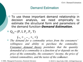


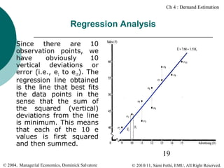
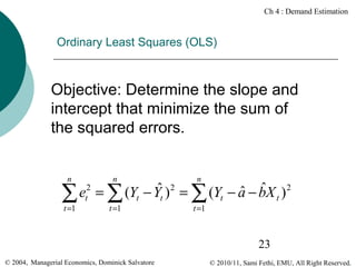
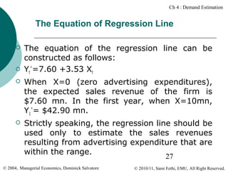
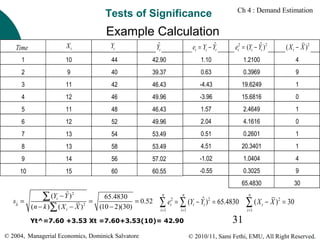
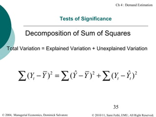
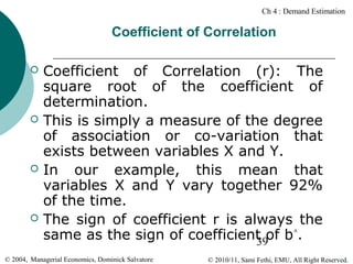
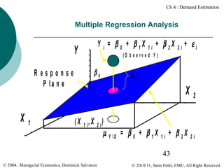
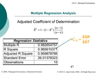
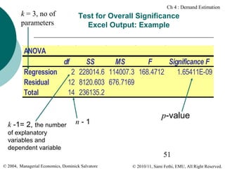
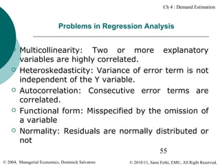
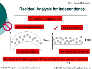
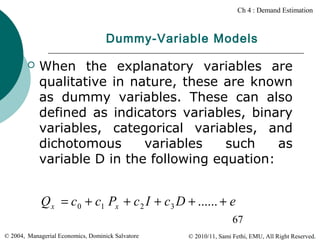
![Ch 4 : Demand Estimation
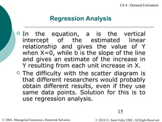
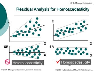
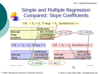
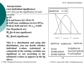
Output by Microfit v4.0w
Ordinary Least Squares Estimation
*******************************************************************************
Dependent variable is LOGN
39 observations used for estimation from 1956 to 1994
*******************************************************************************
Regressor
Coefficient
Standard Error
T-Ratio[Prob]
CON
4.9921
.98407
5.0729[.000]
LOGK
.040394
.012998
3.1078[.004]
LOGW
.024737
.010982
2.2526[.032]
AD
-.9174E-7
.1587E-6
.57798[.567]
LOGP
.026977
.0099796
2.7032[.011]
LOGWT
-.053944
.024279
2.2219[.034]
*******************************************************************************
R-Squared
.82476
F-statistic F( 6, 33)
20.8432[.000]
R-Bar-Squared
.78519
S.E. of Regression
.012467
Residual Sum of Squares
.0048181
Mean of Dependent Variable
10.0098
S.D. of Dependent Variable
.026899
Maximum of Log-likelihood
120.1407
DW-statistic
1.8538
*******************************************************************************
75
© 2004, Managerial Economics, Dominick Salvatore
© 2010/11, Sami Fethi, EMU, All Right Reserved.](https://image.slidesharecdn.com/demandestimation-131215233218-phpapp02/85/Demand-estimation-75-320.jpg)
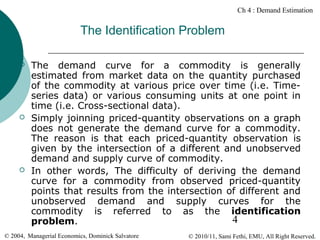
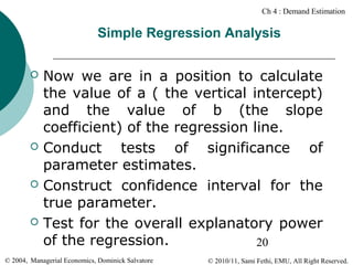
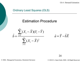
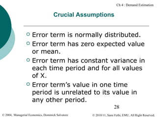
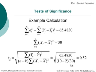
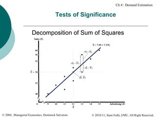
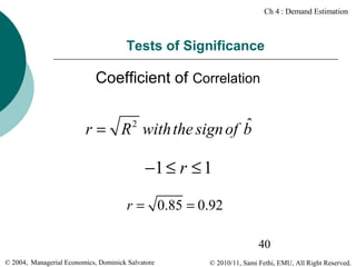
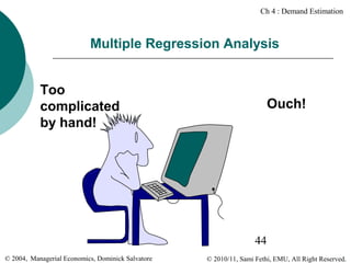
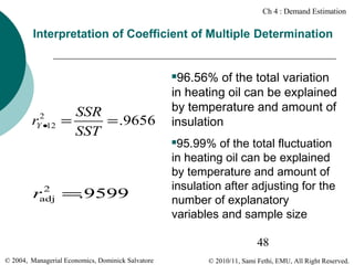
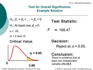
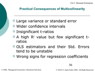
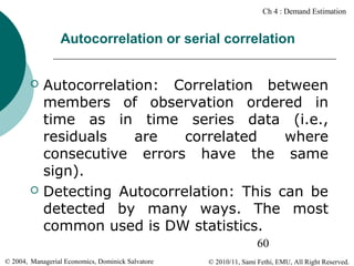
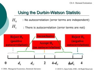
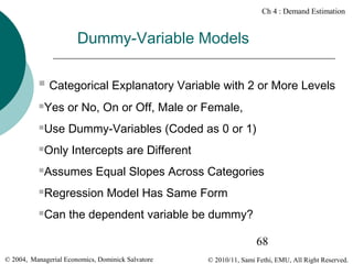
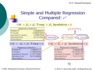
![Ch 4 : Demand Estimation
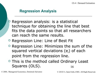
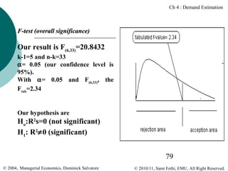
Diagnostic Tests
******************************************************************************
*
*
Test Statistics
*
LM Version
*
F Version
*
******************************************************************************
*
*
*
*
*
* A:Serial Correlation *CHI-SQ( 1)= .051656[.820]*F(1,30)=.039788[.843]*
*
*
*
*
* B:Functional Form
*CHI-SQ( 1)= .056872[.812]*F(1,30)=.043812[.836]*
*
*
*
*
* C:Normality
*CHI-SQ( 2)=
1.2819[.527]*
Not applicable
*
*
*
*
*
* D:Heteroscedasticity *CHI-SQ( 1)=
1.0065[.316]*F( 1,37)=.98022[.329]*
******************************************************************************
*
A:Lagrange
B:Ramsey's
C:Based on
D:Based on
multiplier test of residual serial correlation
RESET test using the square of the fitted values
a test of skewness and kurtosis of residuals
the regression of squared residuals on squared fitted values
76
© 2004, Managerial Economics, Dominick Salvatore
© 2010/11, Sami Fethi, EMU, All Right Reserved.](https://image.slidesharecdn.com/demandestimation-131215233218-phpapp02/85/Demand-estimation-76-320.jpg)
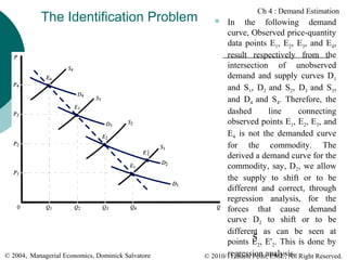
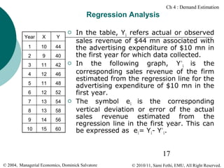
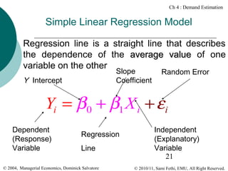
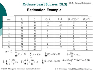
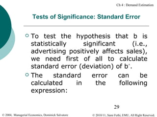
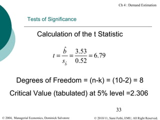
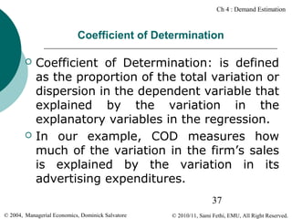
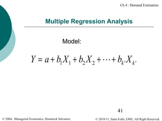
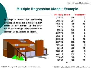
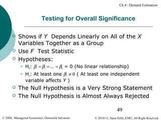
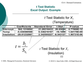
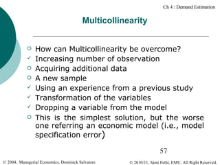
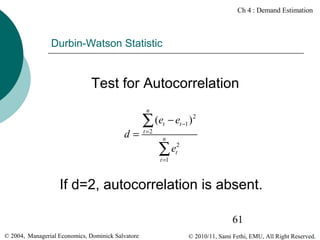
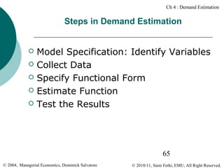
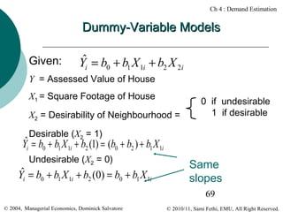
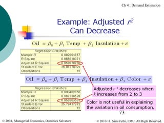
![Ch 4 : Demand Estimation
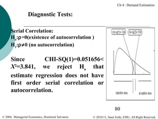
Dependent Variable: LOGN
Explanatory Variables
CON
LOGK
LOGW
AD
LOGP
LOGWT
R2 bar
R2
4.9921
(5.07)
0.40394
(3.10)
0.0247
(2.25)
-0.9174
(-0.577)
0.0269
(2.70)
-0.0539
(-2.22)
0.87
0.83
DW
2.16
SER
0.021
X
2
SC
X
X
2
2
.05165[.820]
FF
05687[.812]
NORM
1.2819[.527]
X2HET
© 2004, Managerial Economics, Dominick Salvatore
77
1.0065[.316]
© 2010/11, Sami Fethi, EMU, All Right Reserved.](https://image.slidesharecdn.com/demandestimation-131215233218-phpapp02/85/Demand-estimation-77-320.jpg)

This document discusses demand estimation through regression analysis. It explains that regression analysis is used to model the relationship between a dependent variable (like quantity demanded) and independent variables (like price, income, etc.). By minimizing the errors between actual data points and the estimated regression line, regression analysis provides the "line of best fit" for estimating demand relationships. The document outlines different marketing research approaches used to collect demand data, including consumer surveys and market experiments. It also discusses the identification problem in directly observing demand from price-quantity data due to shifting supply curves.


