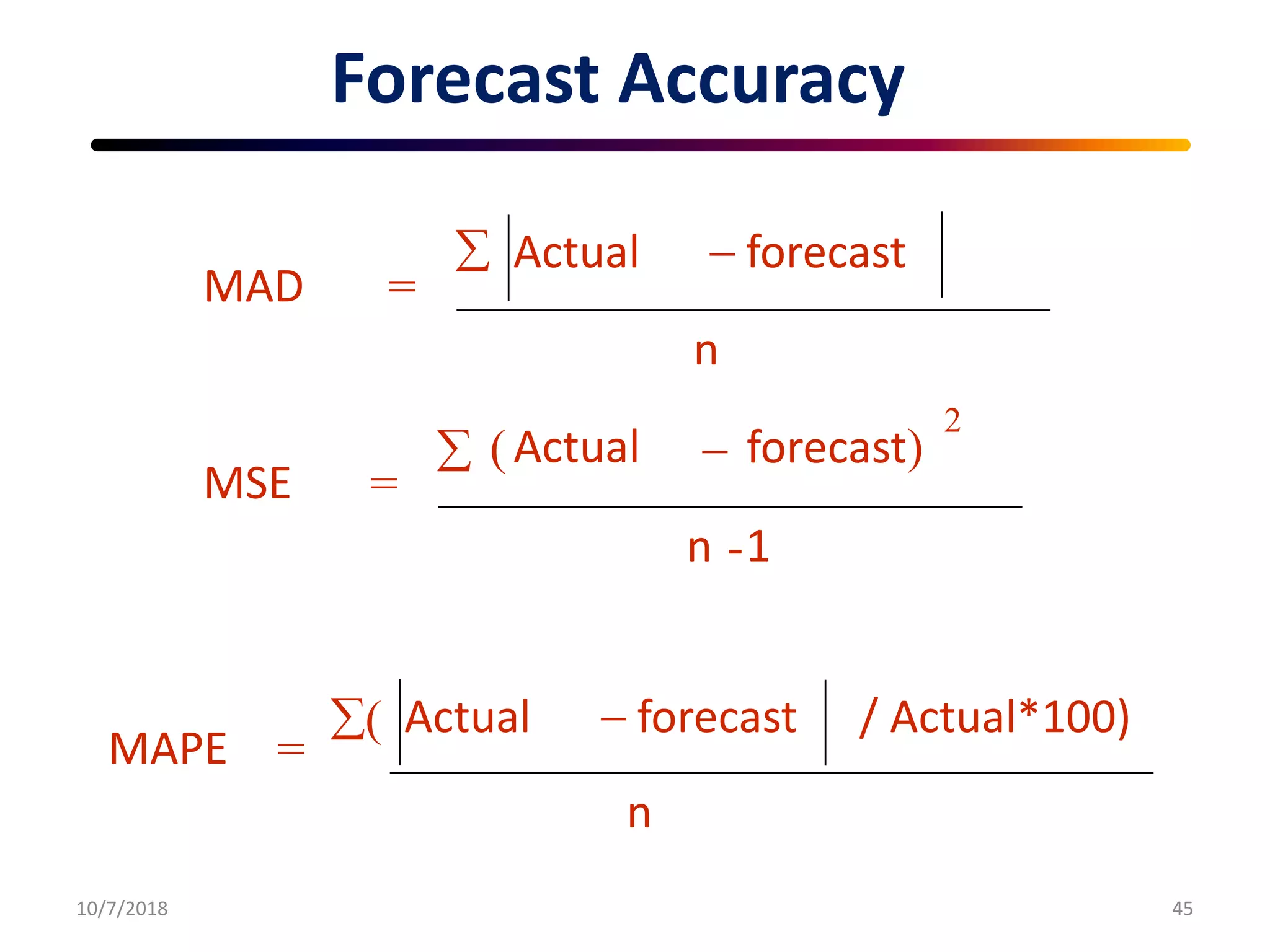
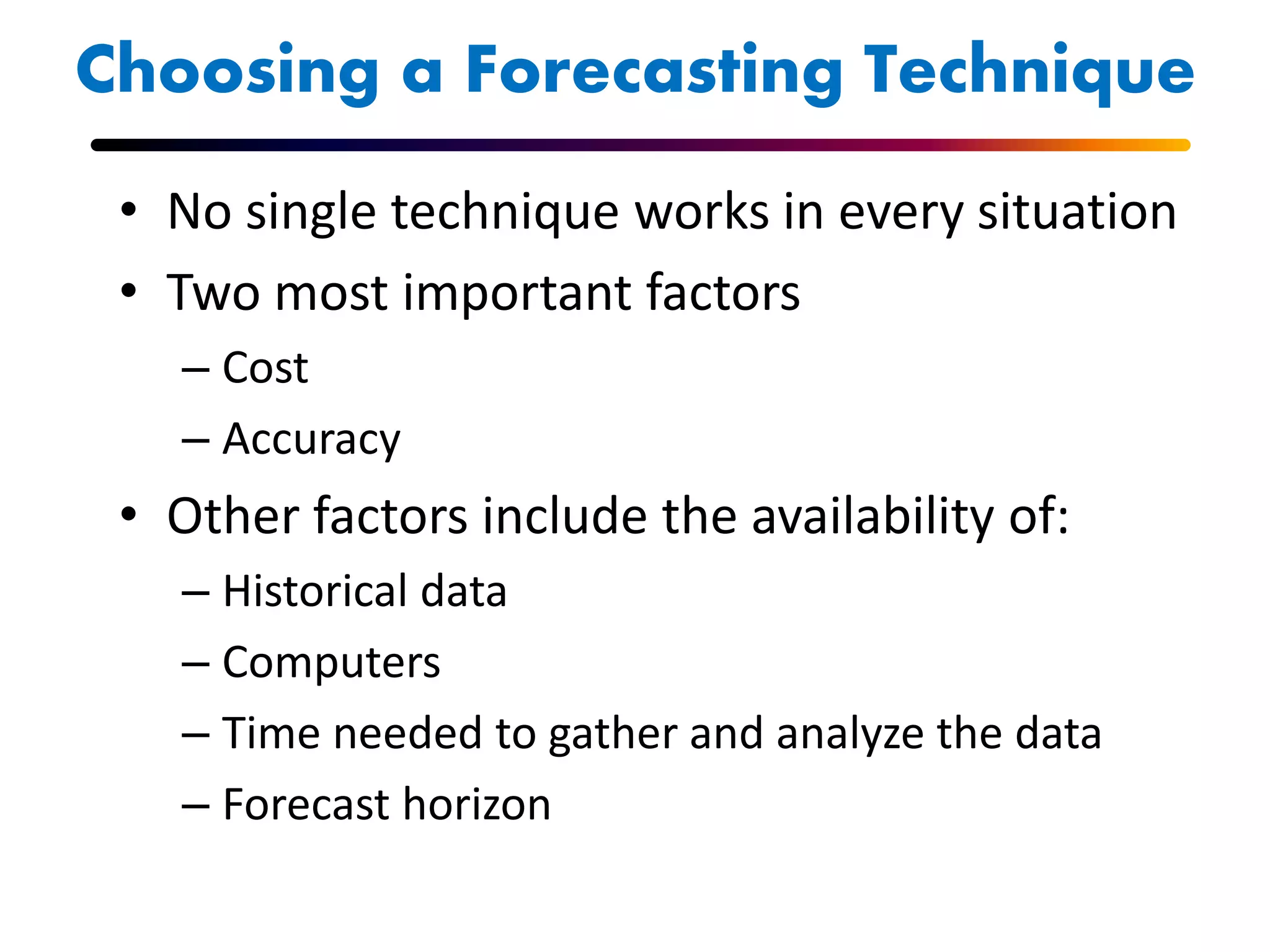
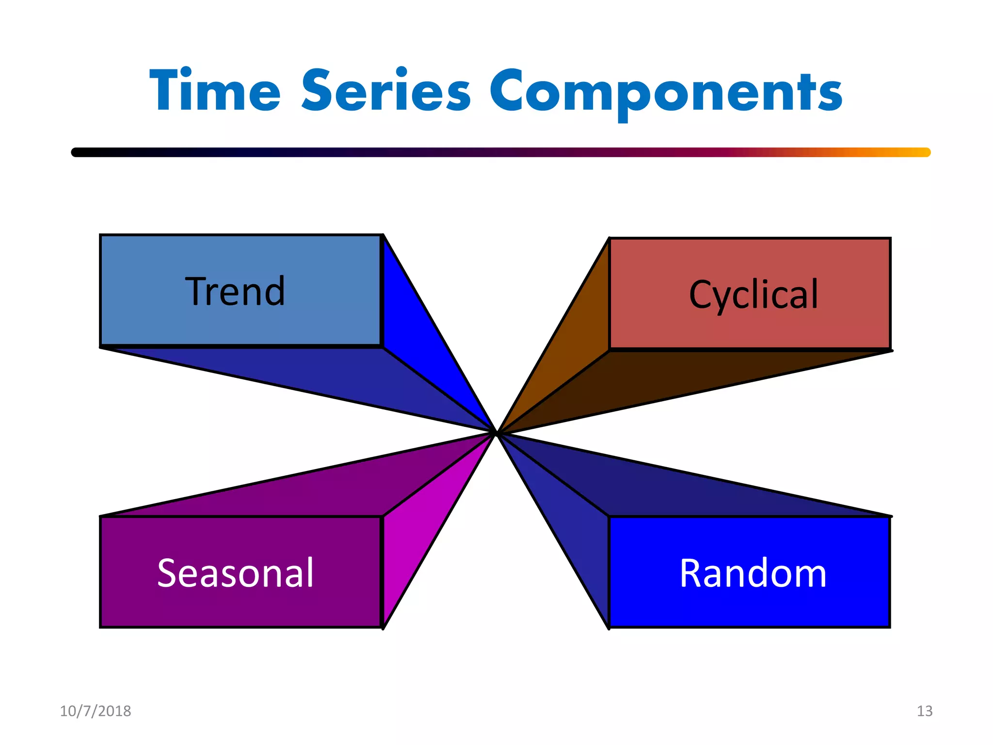
This document discusses various methods for forecasting demand and sales, including quantitative and qualitative techniques. It provides an overview of key forecasting concepts such as time series analysis, moving averages, exponential smoothing, regression analysis, and evaluating forecast accuracy. The document compares different forecasting methods and provides examples of calculating forecasts using techniques like simple and weighted moving averages, exponential smoothing, and linear regression analysis.

1. What We Can Forecast in our
day to day life???

2. past ==> future
I see that you will
get an O this semester.

4. FORECAST:
• A statement about the future value of a variable of
interest such as demand.
• Purpose of demand management is to coordinate and
control all sources of demand so the productive system
can be used efficiently and the product delivered on
time
• Forecasts affect decisions and activities throughout an
organization
– Marketing, sales
– Operations
– Accounting, finance
– Human resources

5. Accounting Cost /profit estimates
Finance Cash flow and funds
Marketing Pricing, promotion, Sales
Operations Inventory, Schedules, MRP,
workloads
Product/service design New products launch
Human Resources Hiring/recruiting/training
Uses of Forecasts

6. Elements of a Good Forecast
Timely
AccurateReliable
Written
/ Data

7. Steps in the Forecasting Process
Step 1 Determine purpose of forecast
Step 2 Establish a time horizon
Step 3 Select a forecasting technique
Step 4 Gather and analyze data
Step 5 Prepare the forecast
Step 6 Monitor the forecast
“The forecast”

8. Types of Forecasts
• Quantitive :(Time series )–
Uses historical data assuming the future will be like the past
• Causal:
Use the relationship between demand and some other factor
to develop forecast
e.g. Price, advertisement etc.
• Qualitative: (Judgmental / Opinion )-
Uses subjective inputs
Rely on judgment and opinion (usually from experts, decision
makers or customer)
• Simulation
– Imitate consumer choices that give rise to demand

9. Quantitative/Time Series Method
• Moving average
– Simple Moving average
– Weighted moving average
• Exponential smoothing
– Simple exponential
– Holt’s model (with trend)
– Winter’s model (with trend and seasonality)
• Regression analysis

10. Qualitative/Judgmental Method
• Opinions
– Sales force opinions
– Executive
– Outside
• Surveys
- Consumer
- Competitor related
• Delphi method
– Opinions of managers and staff

11. Causal Method for forecasting
• Regression analysis

12. Time Series Forecasting
• Forecast based only on past values
– Assumes that factors influencing past and present
will continue influence in future
10/7/2018 12

13. Time Series Components
10/7/2018 13
Trend
Seasonal
Cyclical
Random

14. Time Series Components
10/7/2018 14
Demandforproductorservice
| | | |
1 2 3 4
Year
Average demand
over four years
Seasonal peaks
Trend
component
Actual
demand
Random
variation

15. Trend Component
10/7/2018 15
 Usual starting pointing developing a
forecast.
 Adjusted for seasonal effects, cyclical
elements and random effects.
 Changes due to population, technology,
age, culture, etc.
 Typically several years duration

16. Seasonal Component
10/7/2018 16
 Regular pattern of up and down
fluctuations
 Due to weather, customs, etc.
 Occurs within a single year

17. Cyclical Component
10/7/2018 17
 Repeating up and down movements
 Affected by business cycle, political, and
economic factors
 Multiple years duration
0 5 10 15 20

18. Random Component
10/7/2018 18
 Erratic, unsystematic, ‘residual’ fluctuations
 Due to random variation or unforeseen events
 Short duration and no repeating
M T W T F

19. Naive approach
10/7/2018 19
 Assumes demand in next period is the
same as demand in most recent period
- e.g., If May sales were 48, then June sales will be
48
Sometimes cost effective and efficient

20. Moving Averages
• Simple Moving average – A technique that averages a
number of recent actual values, updated as new values
become available.
• Take the average demand for a defined number of past
periods
• Forecast will lag behind
– Trends
– Seasonality or other cyclicality
MAn =
n
Di
i = 1

n
where
n = number of periods in
the moving average
Di = demand in period i

21. 3-Month Moving Averages
Jan 120
Feb 90
Mar 100
Apr 75
May 110
June 50
July 75
Aug 130
Sept 110
Oct 90
Nov -
ORDERS
MONTH PER MONTH
MA3 =
3
i = 1
 Di
3
=
90 + 110 + 130
3
= 110 orders
for Nov
–
–
–
103.3
88.3
95.0
78.3
78.3
85.0
105.0
110.0
MOVING
AVERAGE

22. 5-Month Moving Averages
Jan 120
Feb 90
Mar 100
Apr 75
May 110
June 50
July 75
Aug 130
Sept 110
Oct 90
Nov -
ORDERS
MONTH PER MONTH
MA5 =
5
i = 1
 Di
5
=
90 + 110 + 130+75+50
5
= 91 orders
for Nov
–
–
–
–
–
99.0
85.0
82.0
88.0
95.0
91.0
MOVING
AVERAGE

23. Smoothing effect
10/7/2018 23
150 –
125 –
100 –
75 –
50 –
25 –
0 – | | | | | | | | | | |
Jan Feb Mar Apr May June July Aug Sept Oct Nov
Actual
Orders
Month
5-month
3-month

24. Weighted moving average
10/7/2018 24
 Adjusts moving average method to more closely reflect data
fluctuations
 Older data usually less important
 Weights based on experience and intuition
WMAn = i = 1
 Wi Di
where
Wi = the weight for period i, between 0
and 100 percent
Di = demand in period i
 Wi = 1.00

25. Weighted moving average
10/7/2018 25
MONTH WEIGHT DATA
August 17% 130
September 33% 110
October 50% 90
WMA3 =
3
i = 1
 Wi Di
= (0.50)(90) + (0.33)(110) + (0.17)(130)
= 103.4 orders
November Forecast

26. Weighted moving average
2610/7/2018
January 10
February 12
March 13
April 16
May 19
June 23
July 26
Actual 3-Month Weighted
Month Shed Sales Moving Average
[(3 x 16) + (2 x 13) + (12)]/6 = 141/3
[(3 x 19) + (2 x 16) + (13)]/6 = 17
[(3 x 23) + (2 x 19) + (16)]/6 = 201/2
10
12
13
[(3 x 13) + (2 x 12) + (10)]/6 = 121/6

27. Weighted moving average
2710/7/2018
30 –
25 –
20 –
15 –
10 –
5 –
Salesdemand
| | | | | | | | | | | |
J F M A M J J A S O N D
Actual
sales
Moving
average
Weighted
moving
average

28. Exponential Smoothing
2810/7/2018
• Form of weighted moving average
– Weights decline exponentially
– Most recent data weighted most
• Requires smoothing constant (α)
– Ranges from 0 to 1
– Subjectively chosen
• Involves little record keeping of past data

29. Exponential Smoothing
2910/7/2018
New forecast = last period’s forecast
+ a (last period’s actual demand
– last period’s forecast)
Ft = Ft – 1 + a(At – 1 - Ft – 1)
where Ft = new forecast
Ft – 1 = previous forecast
a = smoothing (or weighting)
constant (0  a  1)

30. Period Actual Alpha = 0.1 Error Alpha = 0.4 Error
1 42
2 40 42 -2.00 42 -2
3 43 41.8 1.20 41.2 1.8
4 40 41.92 -1.92 41.92 -1.92
5 41 41.73 -0.73 41.15 -0.15
6 39 41.66 -2.66 41.09 -2.09
7 46 41.39 4.61 40.25 5.75
8 44 41.85 2.15 42.55 1.45
9 45 42.07 2.93 43.13 1.87
10 38 42.36 -4.36 43.88 -5.88
11 40 41.92 -1.92 41.53 -1.53
12 41.73 40.92
Example - Exponential Smoothing

31. Impact of The Value of a

32. Choosing appropriate Value of ᾳ
 If real demand is stable: small ᾳ
 If real demand is rapidly increasing or
decreasing: large ᾳ to try to keep up with the
change.
Two Approaches to control the value of ᾳ:
Two or more predetermined values of ᾳ
Computed values for ᾳ

33. Choosing appropriate Value of ᾳ
Two or more predetermined values of ᾳ
If error is large: ᾳ ≥ 0.8
If error is small: ᾳ ≤ 0.2
Computed values for ᾳ
Tracking ᾳ = Exponentially smoothed actual
error divided by exponentially smoothed
absolute error.

34. Trend effects in exponential smoothing
 To correct the trend to smoothing constant are required:
– Smoothing constant ᾳ and smoothing constant δ
– δ reduces the impact of errors
– For first time, trend value must be entered manually.
– This trend value can be educated guess or a computation based on
observed past data
FITt-1 = Ft-1 + Tt-1
Ft = FITt-1 + ᾳ (At -1 - FITt-1 )
Tt = Tt-1 + δ (Ft - FITt-1 )

36. Linear Regression Analysis
 Useful for long term forecasting of major
occurrences and aggregate planning.
e.g. very useful for product families.
 Used for both time series forecasting and causal
forecasting.
 Time series forecasting: If dependent variable
changes as a result of time
 Casual forecasting: If one variable changes because
of change in another variable.

37. Linear Regression Analysis
• Ft = Forecast for period t (Dependent Variable)
• t = Specified number of time periods
• a = Y intercept
• b = Slope of the line
Ft = a + bt
0 1 2 3 4 5 t
Ft
b =
n (xy) - y
n x2 - ( x)2
x

a =
y - b x
n


38. Example
x y
Week x2
Sales xy
1 1 150 150
2 4 157 314
3 9 162 486
4 16 166 664
5 25 177 885
 x = 15 x2
= 55  y = 812  xy = 2499
(x)2
= 225

39. Calculation
y = 143.5 + 6.3t
a =
812 - 6.3(15)
5
=
b =
5 (2499) - 15(812)
5(55) - 225
=
12495 -12180
275 -225
= 6.3
143.5

40. Correlation Analysis
 How strong is the linear relationship between the
variables?
- a measure of the strength of the relationship between
independent and dependent variables
 Coefficient of correlation, r, measures degree of
association
 Values range from -1 to +1
r =
nxy - xy
[nx2 - (x)2][ny2 - (y)2]

41. Correlation Analysis
10/7/2018 41
y
x(a) Perfect positive
correlation:
r = +1
y
x
(c) No correlation:
r = 0
y
x(b) Positive
correlation:
0 < r < 1
y
x
(d) Perfect negative
correlation:
r = -1

42. Correlation Analysis
10/7/2018 42
x y
Week Sales
1 150
2 157
3 162
4 166
5 177

43. Forecast Accuracy
 Error - difference between actual value and predicted
value
 Mean Absolute Deviation (MAD)
- Average absolute error
 Mean Squared Error (MSE)
- Average of squared error
 Mean Absolute Percent Error (MAPE)
- Average absolute percent error

44. Forecast Accuracy
 MAD
– Easy to compute
– Weights errors linearly
 MSE
– Squares error
– More weight to large errors
 MAPE
– Puts errors in percent

45. Forecast Accuracy
10/7/2018 45
MAD =
Actual forecast
n
MSE =
Actual forecast)
-1
2

n
(
MAPE =
Actual forecast
n
/ Actual*100)(

46. Example
Period Actual Forecast (A-F) |A-F| (A-F)^2 (|A-F|/Actual)*100
1 217 215 2 2 4 0.92
2 213 216 -3 3 9 1.41
3 216 215 1 1 1 0.46
4 210 214 -4 4 16 1.90
5 213 211 2 2 4 0.94
6 219 214 5 5 25 2.28
7 216 217 -1 1 1 0.46
8 212 216 -4 4 16 1.89
-2 22 76 10.26
MAD= 2.75
MSE= 10.86
MAPE= 1.28

47. Mean absolute deviation
MAD =
A - F
n
t t
t=1
n

1 MAD 0.8 standard deviation
1 standard deviation 1.25 MAD


• The ideal MAD is zero which would mean there
is no forecasting error
• The larger the MAD, the less the accurate the
resulting model

48. Tracking Signal
Tracking signal =
(Actual-forecast)
MAD

•Tracking signal
–Ratio of cumulative error to MAD

49. Choosing a Forecasting Technique
• No single technique works in every situation
• Two most important factors
– Cost
– Accuracy
• Other factors include the availability of:
– Historical data
– Computers
– Time needed to gather and analyze the data
– Forecast horizon

50. Thank you!!
