Downloaded 54 times
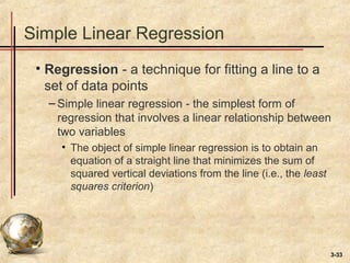
![3-11
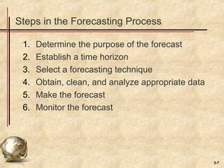
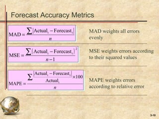
Forecast Error Calculation
Period
Actual
(A)
Forecast
(F)
(A-F)
Error |Error| Error2
[|Error|/Actual]x100
1 107 110 -3 3 9 2.80%
2 125 121 4 4 16 3.20%
3 115 112 3 3 9 2.61%
4 118 120 -2 2 4 1.69%
5 108 109 1 1 1 0.93%
Sum 13 39 11.23%
n = 5 n-1 = 4 n = 5
MAD MSE MAPE
= 2.6 = 9.75 = 2.25%](https://image.slidesharecdn.com/modifiedchap003-140417184724-phpapp02/85/Modified-chap003-11-320.jpg)

This document discusses various forecasting techniques. It begins by defining a forecast and explaining that forecasts are used to help managers plan systems and use of systems. Common features of all forecasts are discussed, as are elements of a good forecast. The forecasting process involves determining purpose, time horizon, technique, data analysis, making the forecast, and monitoring. Accuracy is important and can be measured using MAD, MSE, and MAPE. Qualitative and quantitative techniques are covered, along with judgmental, time series, and associative models. Specific time series techniques like naive, moving average, exponential smoothing, and trend/seasonal adjustments are explained. The document concludes by discussing using forecast information reactively or proactively.