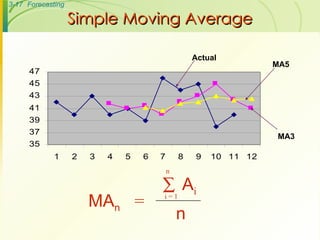
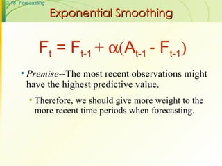
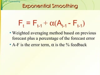
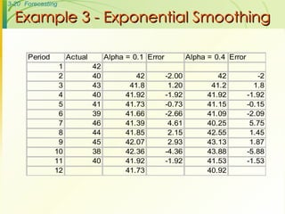
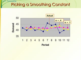
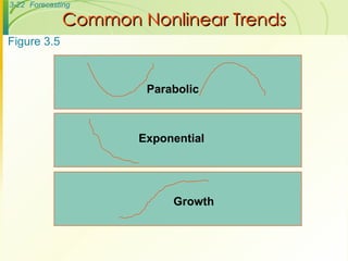
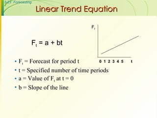
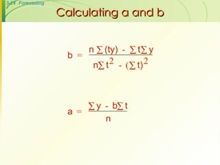
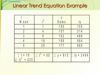
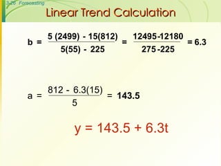
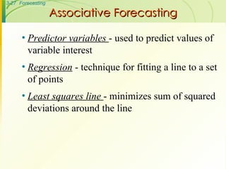
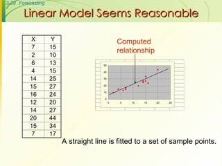
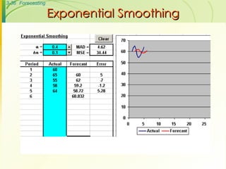
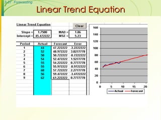
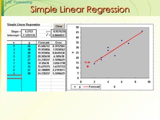
The document discusses various forecasting techniques including judgmental forecasts, time series forecasts, naive forecasts, moving averages, exponential smoothing, linear trends, and associative forecasts using simple linear regression. It describes the basic approaches and formulas for each technique and discusses factors to consider when choosing a forecasting method such as cost, accuracy, data availability, and forecast horizon.

1. William J. Stevenson Operations Management 8 th edition

2. CHAPTER 3 Forecasting McGraw-Hill/Irwin Operations Management, Eighth Edition, by William J. Stevenson Copyright © 2005 by The McGraw-Hill Companies, Inc. All rights reserved.

3. FORECAST : A statement about the future value of a variable of interest such as demand. Forecasts affect decisions and activities throughout an organization Accounting, finance Human resources Marketing MIS Operations Product / service design

4. Uses of Forecasts New products and services Product/service design Schedules, MRP, workloads Operations IT/IS systems, services MIS Pricing, promotion, strategy Marketing Hiring/recruiting/training Human Resources Cash flow and funding Finance Cost/profit estimates Accounting

5. Assumes causal system past ==> future Forecasts rarely perfect because of randomness Forecasts more accurate for groups vs. individuals Forecast accuracy decreases as time horizon increases I see that you will get an A this semester.

6. Elements of a Good Forecast Timely Accurate Reliable Meaningful Written Easy to use

7. Steps in the Forecasting Process Step 1 Determine purpose of forecast Step 2 Establish a time horizon Step 3 Select a forecasting technique Step 4 Gather and analyze data Step 5 Prepare the forecast Step 6 Monitor the forecast “ The forecast”

8. Types of Forecasts Judgmental - uses subjective inputs Time series - uses historical data assuming the future will be like the past Associative models - uses explanatory variables to predict the future

9. Judgmental Forecasts Executive opinions Sales force opinions Consumer surveys Outside opinion Delphi method Opinions of managers and staff Achieves a consensus forecast

10. Time Series Forecasts Trend - long-term movement in data Seasonality - short-term regular variations in data Cycle – wavelike variations of more than one year’s duration Irregular variations - caused by unusual circumstances Random variations - caused by chance

11. Forecast Variations Trend Irregular variation Seasonal variations 90 89 88 Figure 3.1 Cycles

12. Naive Forecasts The forecast for any period equals the previous period’s actual value. Uh, give me a minute.... We sold 250 wheels last week.... Now, next week we should sell....

13. Simple to use Virtually no cost Quick and easy to prepare Data analysis is nonexistent Easily understandable Cannot provide high accuracy Can be a standard for accuracy Naïve Forecasts

14. Stable time series data F(t) = A(t-1) Seasonal variations F(t) = A(t-n) Data with trends F(t) = A(t-1) + (A(t-1) – A(t-2)) Uses for Naïve Forecasts

15. Techniques for Averaging Moving average Weighted moving average Exponential smoothing

16. Moving Averages Moving average – A technique that averages a number of recent actual values, updated as new values become available. Weighted moving average – More recent values in a series are given more weight in computing the forecast. MA n = n A i i = 1  n

17. Simple Moving Average Actual MA3 MA5 MA n = n A i i = 1  n

18. Exponential Smoothing Premise --The most recent observations might have the highest predictive value. Therefore, we should give more weight to the more recent time periods when forecasting. F t = F t-1 +  ( A t-1 - F t-1 )

19. Exponential Smoothing Weighted averaging method based on previous forecast plus a percentage of the forecast error A-F is the error term,  is the % feedback F t = F t-1 +  ( A t-1 - F t-1 )

20. Example 3 - Exponential Smoothing

21. Picking a Smoothing Constant  .1  .4 Actual

22. Common Nonlinear Trends Figure 3.5 Parabolic Exponential Growth

23. Linear Trend Equation F t = Forecast for period t t = Specified number of time periods a = Value of F t at t = 0 b = Slope of the line F t = a + bt 0 1 2 3 4 5 t F t

24. Calculating a and b b = n (ty) - t y n t 2 - ( t) 2 a = y - b t n       

25. Linear Trend Equation Example

26. Linear Trend Calculation y = 143.5 + 6.3t a = 812 - 6.3(15) 5 = b = 5 (2499) - 15(812) 5(55) - 225 = 12495 - 12180 275 - 225 = 6.3 143.5

27. Associative Forecasting Predictor variables - used to predict values of variable interest Regression - technique for fitting a line to a set of points Least squares line - minimizes sum of squared deviations around the line

28. Linear Model Seems Reasonable A straight line is fitted to a set of sample points. Computed relationship

29. Forecast Accuracy Error - difference between actual value and predicted value Mean Absolute Deviation (MAD) Average absolute error Mean Squared Error (MSE) Average of squared error Mean Absolute Percent Error (MAPE) Average absolute percent error

30. MAD, MSE, and MAPE MAD = Actual forecast   n MSE = Actual forecast ) - 1 2   n ( MAPE = Actual forecast  n / Actual*100) 

31. Example 10

32. Controlling the Forecast Control chart A visual tool for monitoring forecast errors Used to detect non-randomness in errors Forecasting errors are in control if All errors are within the control limits No patterns, such as trends or cycles, are present

33. Sources of Forecast errors Model may be inadequate Irregular variations Incorrect use of forecasting technique

34. Tracking Signal Tracking signal Ratio of cumulative error to MAD Bias – Persistent tendency for forecasts to be Greater or less than actual values. Tracking signal = ( Actual - forecast ) MAD 

35. Choosing a Forecasting Technique No single technique works in every situation Two most important factors Cost Accuracy Other factors include the availability of: Historical data Computers Time needed to gather and analyze the data Forecast horizon

36. Exponential Smoothing

37. Linear Trend Equation

38. Simple Linear Regression