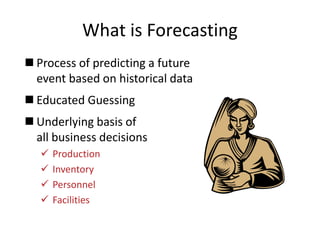
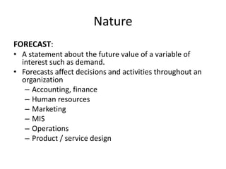
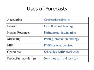
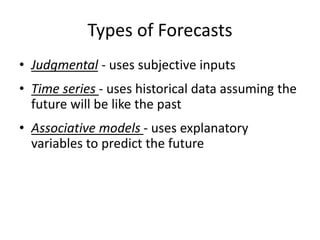
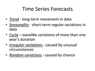
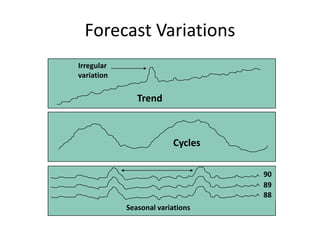
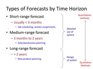
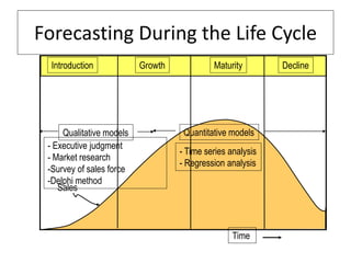
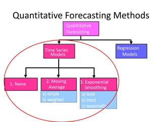
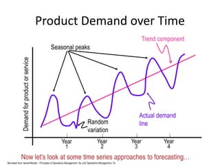
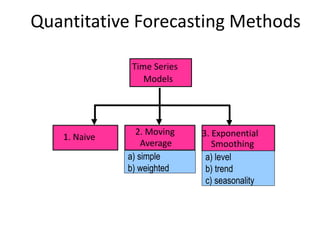
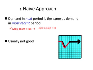
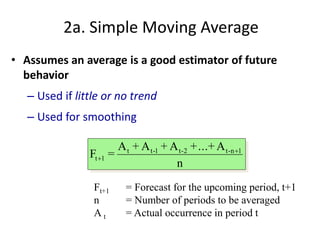
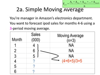
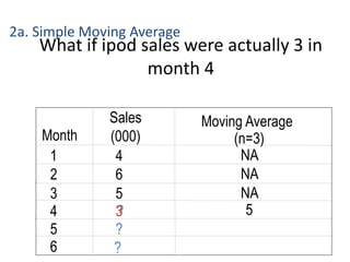
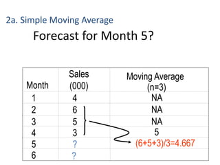
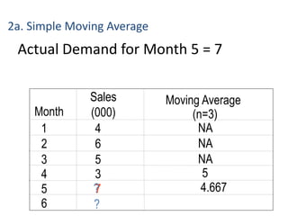
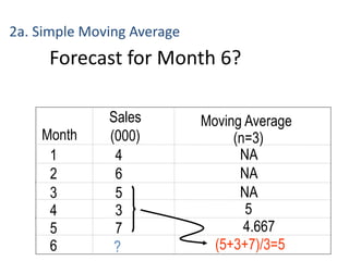
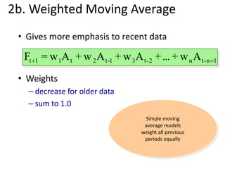
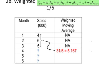
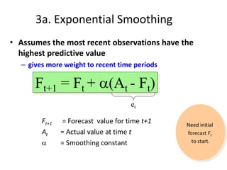
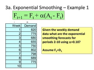
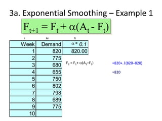
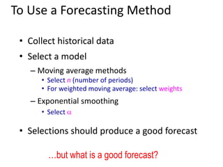
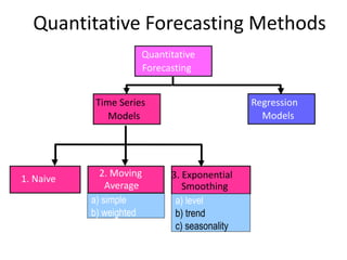
This document discusses forecasting methods used in production and operations management. It defines forecasting as predicting future values based on historical data. The key types of forecasts discussed are judgmental forecasts using subjective inputs, time series forecasts using historical data patterns, and associative models using explanatory variables. Time series methods covered include simple moving averages, weighted moving averages, and exponential smoothing. Exponential smoothing gives more weight to recent periods to generate forecasts. Quantitative forecasting methods are chosen based on the forecast horizon and data available.

1. Course: MBA
Subject: Production & Operation
Management
Unit:1.3
Forecasting

2. Forecast
• Nature
• Types
• Factors affecting forecasting
• Models

3. What is Forecasting
 Process of predicting a future
event based on historical data
 Educated Guessing
 Underlying basis of
all business decisions
 Production
 Inventory
 Personnel
 Facilities

4. Importance of Forecasting in PM &OM
• Departments throughout the organization depend on
forecasts to formulate and execute their plans.
• Finance needs forecasts to project cash flows and
capital requirements.
• Human resources need forecasts to anticipate hiring
needs.
• Production needs forecasts to plan production levels,
workforce, material requirements, inventories, etc.

5. Importance of Forecasting in PM &OM
• Demand is not the only variable of interest to
forecasters.
• Manufacturers also forecast worker absenteeism,
machine availability, material costs,
transportation and production lead times, etc.
• Besides demand, service providers are also
interested in forecasts of population, of other
demographic variables, of weather, etc.

6. Nature
FORECAST:
• A statement about the future value of a variable of
interest such as demand.
• Forecasts affect decisions and activities throughout an
organization
– Accounting, finance
– Human resources
– Marketing
– MIS
– Operations
– Product / service design

7. Uses of Forecasts
Accounting Cost/profit estimates
Finance Cash flow and funding
Human Resources Hiring/recruiting/training
Marketing Pricing, promotion, strategy
MIS IT/IS systems, services
Operations Schedules, MRP, workloads
Product/service design New products and services

8. • Assumes causal system
past ==> future
• Forecasts rarely perfect because of
randomness
• Forecasts more accurate for
groups vs. individuals
• Forecast accuracy decreases
as time horizon increases
I see that you will
get an A this semester.

9. Elements of a Good Forecast
Timely
AccurateReliable
Written

10. Steps in the Forecasting Process
Step 1 Determine purpose of forecast
Step 2 Establish a time horizon
Step 3 Select a forecasting technique
Step 4 Gather and analyze data
Step 5 Prepare the forecast
Step 6 Monitor the forecast
“The forecast”

11. Types of Forecasts
• Judgmental - uses subjective inputs
• Time series - uses historical data assuming the
future will be like the past
• Associative models - uses explanatory
variables to predict the future

12. Judgmental Forecasts
• Executive opinions
• Sales force opinions
• Consumer surveys
• Outside opinion
• Delphi method
– Opinions of managers and staff
– Achieves a consensus forecast

13. Time Series Forecasts
• Trend - long-term movement in data
• Seasonality - short-term regular variations in
data
• Cycle – wavelike variations of more than one
year’s duration
• Irregular variations - caused by unusual
circumstances
• Random variations - caused by chance

14. Forecast Variations
Trend
Irregular
variation
Seasonal variations
90
89
88
Cycles

15. Types of Forecasts by Time Horizon
• Short-range forecast
– Usually < 3 months
• Job scheduling, worker assignments
• Medium-range forecast
– 3 months to 2 years
• Sales/production planning
• Long-range forecast
– > 2 years
• New product planning
Quantitative
methods
Qualitative
Methods
Detailed
use of
system
Design
of system

16. Forecasting During the Life Cycle
Introduction Growth Maturity Decline
Sales
Time
Quantitative models
- Time series analysis
- Regression analysis
Qualitative models
- Executive judgment
- Market research
-Survey of sales force
-Delphi method

17. Qualitative Forecasting Methods
Qualitative
Forecasting
Models
Market
Research/
Survey
Sales
Force
Composite
Executive
Judgement
Delphi
Method
Smoothing

18. Qualitative Methods
Briefly, the qualitative methods are:
Executive Judgment: Opinion of a group of high level experts or managers is
pooled
Sales Force Composite: Each regional salesperson provides his/her sales
estimates. Those forecasts are then reviewed to make sure they are realistic.
All regional forecasts are then pooled at the district and national levels to
obtain an overall forecast.
Market Research/Survey: Solicits input from customers pertaining to their future
purchasing plans. It involves the use of questionnaires, consumer panels and
tests of new products and services.
• .

19. Delphi Method
Delphi Method: As opposed to regular panels where the individuals involved are
in direct communication, this method eliminates the effects of group potential
dominance of the most vocal members. The group involves individuals from
inside as well as outside the organization.
Typically, the procedure consists of the following steps:
Each expert in the group makes his/her own forecasts in form of statements
 The coordinator collects all group statements and summarizes them
 The coordinator provides this summary and gives another set of
questions to each group member including feedback as to the input of
other experts.
 The above steps are repeated until a consensus is reached.
• .

20. Quantitative Forecasting Methods
Quantitative
Forecasting
Regression
Models
2. Moving
Average
1. Naive
Time Series
Models
3. Exponential
Smoothing
a) simple
b) weighted
a) level
b) trend
c) seasonality

21. Time Series Models
• Try to predict the future based on past data
– Assume that factors influencing the past will
continue to influence the future

22. Time Series Models: Components
Random
Seasonal
Trend
Composite

23. Product Demand over Time
Year
1
Year
2
Year
3
Year
4
Demandforproductorservice

24. Product Demand over Time
Year
1
Year
2
Year
3
Year
4
Demandforproductorservice
Trend component
Actual demand
line
Seasonal peaks
Random
variation
Now let’s look at some time series approaches to forecasting…
Borrowed from Heizer/Render - Principles of Operations Management, 5e, and Operations Management, 7e

25. Quantitative Forecasting Methods
Quantitative
Models
2. Moving
Average
1. Naive
Time Series
Models
3. Exponential
Smoothing
a) simple
b) weighted
a) level
b) trend
c) seasonality

26. 1. Naive Approach
 Demand in next period is the same as demand
in most recent period
May sales = 48 →
 Usually not good
June forecast = 48

27. Naïve Approach
• Simple to use
• Virtually no cost
• Quick and easy to prepare
• Data analysis is nonexistent
• Easily understandable
• Cannot provide high accuracy
• Can be a standard for accuracy

28. 2a. Simple Moving Average
n
A+...+A+A+A
=F 1n-t2-t1-tt
1t


• Assumes an average is a good estimator of future
behavior
– Used if little or no trend
– Used for smoothing
Ft+1 = Forecast for the upcoming period, t+1
n = Number of periods to be averaged
A t = Actual occurrence in period t

29. 2a. Simple Moving Average
You’re manager in Amazon’s electronics department.
You want to forecast ipod sales for months 4-6 using a
3-period moving average.
n
A+...+A+A+A
=F 1n-t2-t1-tt
1t


Month
Sales
(000)
1 4
2 6
3 5
4 ?
5 ?
6 ?

30. 2a. Simple Moving Average
Month
Sales
(000)
Moving Average
(n=3)
1 4 NA
2 6 NA
3 5 NA
4 ?
5 ?
(4+6+5)/3=5
6 ?
n
A+...+A+A+A
=F 1n-t2-t1-tt
1t


You’re manager in Amazon’s electronics department.
You want to forecast ipod sales for months 4-6 using a
3-period moving average.

31. What if ipod sales were actually 3 in
month 4
Month
Sales
(000)
Moving Average
(n=3)
1 4 NA
2 6 NA
3 5 NA
4 3
5 ?
5
6 ?
2a. Simple Moving Average
?

32. Forecast for Month 5?
Month
Sales
(000)
Moving Average
(n=3)
1 4 NA
2 6 NA
3 5 NA
4 3
5 ?
5
6 ?
(6+5+3)/3=4.667
2a. Simple Moving Average

33. Actual Demand for Month 5 = 7
Month
Sales
(000)
Moving Average
(n=3)
1 4 NA
2 6 NA
3 5 NA
4 3
5 7
5
6 ?
4.667
2a. Simple Moving Average
?

34. Forecast for Month 6?
Month
Sales
(000)
Moving Average
(n=3)
1 4 NA
2 6 NA
3 5 NA
4 3
5 7
5
6 ?
4.667
(5+3+7)/3=5
2a. Simple Moving Average

35. • Gives more emphasis to recent data
• Weights
– decrease for older data
– sum to 1.0
2b. Weighted Moving Average
1n-tn2-t31-t2t11t Aw+...+Aw+Aw+Aw=F 
Simple moving
average models
weight all previous
periods equally

36. 2b. Weighted Moving Average: 3/6, 2/6,
1/6
Month Weighted
Moving
Average
1 4 NA
2 6 NA
3 5 NA
4 31/6 = 5.167
5
6 ?
?
?
1n-tn2-t31-t2t11t Aw+...+Aw+Aw+Aw=F 
Sales
(000)

37. 2b. Weighted Moving Average: 3/6, 2/6,
1/6
Month Sales
(000)
Weighted
Moving
Average
1 4 NA
2 6 NA
3 5 NA
4 3 31/6 = 5.167
5 7
6
25/6 = 4.167
32/6 = 5.333
1n-tn2-t31-t2t11t Aw+...+Aw+Aw+Aw=F 

38. 3a. Exponential Smoothing
• Assumes the most recent observations have the
highest predictive value
– gives more weight to recent time periods
Ft+1 = Ft + a(At - Ft)
et
Ft+1 = Forecast value for time t+1
At = Actual value at time t
a = Smoothing constant
Need initial
forecast Ft
to start.

39. 3a. Exponential Smoothing – Example 1
Week Demand
1 820
2 775
3 680
4 655
5 750
6 802
7 798
8 689
9 775
10
Given the weekly demand
data what are the exponential
smoothing forecasts for
periods 2-10 using a=0.10?
Assume F1=D1
Ft+1 = Ft + a(At - Ft)
i Ai

40. Week Demand 0.1 0.6
1 820 820.00 820.00
2 775 820.00 820.00
3 680 815.50 793.00
4 655 801.95 725.20
5 750 787.26 683.08
6 802 783.53 723.23
7 798 785.38 770.49
8 689 786.64 787.00
9 775 776.88 728.20
10 776.69 756.28
Ft+1 = Ft + a(At - Ft)
3a. Exponential Smoothing – Example 1
a =
F2 = F1+ a(A1–F1) =820+.1(820–820)
=820
i Ai Fi

41. Week Demand 0.1 0.6
1 820 820.00 820.00
2 775 820.00 820.00
3 680 815.50 793.00
4 655 801.95 725.20
5 750 787.26 683.08
6 802 783.53 723.23
7 798 785.38 770.49
8 689 786.64 787.00
9 775 776.88 728.20
10 776.69 756.28
Ft+1 = Ft + a(At - Ft)
3a. Exponential Smoothing – Example 1
a =
F3 = F2+ a(A2–F2) =820+.1(775–820)
=815.5
i Ai Fi

42. Week Demand 0.1 0.6
1 820 820.00 820.00
2 775 820.00 820.00
3 680 815.50 793.00
4 655 801.95 725.20
5 750 787.26 683.08
6 802 783.53 723.23
7 798 785.38 770.49
8 689 786.64 787.00
9 775 776.88 728.20
10 776.69 756.28
Ft+1 = Ft + a(At - Ft)
This process
continues
through week 10
3a. Exponential Smoothing – Example 1
a =
i Ai Fi

43. Week Demand 0.1 0.6
1 820 820.00 820.00
2 775 820.00 820.00
3 680 815.50 793.00
4 655 801.95 725.20
5 750 787.26 683.08
6 802 783.53 723.23
7 798 785.38 770.49
8 689 786.64 787.00
9 775 776.88 728.20
10 776.69 756.28
Ft+1 = Ft + a(At - Ft)
What if the
a constant
equals 0.6
3a. Exponential Smoothing – Example 1
a = a =
i Ai Fi

44. Month Demand 0.3 0.6
January 120 100.00 100.00
February 90 106.00 112.00
March 101 101.20 98.80
April 91 101.14 100.12
May 115 98.10 94.65
June 83 103.17 106.86
July 97.12 92.54
August
September
Ft+1 = Ft + a(At - Ft)
What if the
a constant
equals 0.6
3a. Exponential Smoothing – Example 2
a = a =
i Ai Fi

45. Company A, a personal computer producer
purchases generic parts and assembles them to
final product. Even though most of the orders
require customization, they have many common
components. Thus, managers of Company A need
a good forecast of demand so that they can
purchase computer parts accordingly to minimize
inventory cost while meeting acceptable service
level. Demand data for its computers for the past 5
months is given in the following table.
3a. Exponential Smoothing – Example 3

46. Month Demand 0.3 0.5
January 80 84.00 84.00
February 84 82.80 82.00
March 82 83.16 83.00
April 85 82.81 82.50
May 89 83.47 83.75
June 85.13 86.38
July ?? ??
Ft+1 = Ft + a(At - Ft)
What if the
a constant
equals 0.5
3a. Exponential Smoothing – Example 3
a = a =
i Ai Fi

47. • How to choose α
– depends on the emphasis you want to place on
the most recent data
• Increasing α makes forecast more sensitive to
recent data
3a. Exponential Smoothing

48. Ft+1 = a At + a(1- a) At - 1 + a(1- a)2At - 2 + ...
Forecast Effects of
Smoothing Constant a
Weights
Prior Period
a
2 periods ago
a(1 - a)
3 periods ago
a(1 - a)2
a=
a= 0.10
a= 0.90
10% 9% 8.1%
90% 9% 0.9%
Ft+1 = Ft + a (At - Ft)
or
w1 w2 w3

49. • Collect historical data
• Select a model
– Moving average methods
• Select n (number of periods)
• For weighted moving average: select weights
– Exponential smoothing
• Select a
• Selections should produce a good forecast
To Use a Forecasting Method
…but what is a good forecast?

50. A Good Forecast
Has a small error
 Error = Demand - Forecast

51. Measures of Forecast Error
b. MSE = Mean Squared Error  
n
F-A
=MSE
n
1=t
2
tt
MAD =
A - F
n
t t
t=1
n

et
 Ideal values =0 (i.e., no forecasting error)
MSE=RMSEc. RMSE = Root Mean Squared Error
a. MAD = Mean Absolute Deviation

52. MAD Example
Month Sales Forecast
1 220 n/a
2 250 255
3 210 205
4 300 320
5 325 315
What is the MAD value given the forecast
values in the table below?
MAD =
A - F
n
t t
t=1
n

5
5
20
10
|At – Ft|
FtAt
= 40
= 40
4
=10

53. MSE/RMSE Example
Month Sales Forecast
1 220 n/a
2 250 255
3 210 205
4 300 320
5 325 315
What is the MSE value?
5
5
20
10
|At – Ft|
FtAt
= 550
4
=137.5
(At – Ft)2
25
25
400
100
= 550
 
n
F-A
=MSE
n
1=t
2
tt
RMSE = √137.5
=11.73

54. Measures of Error
t At Ft et |et| et
2
Jan 120 100 20 20 400
Feb 90 106 256
Mar 101 102
April 91 101
May 115 98
June 83 103
1. Mean Absolute Deviation
(MAD)
n
e
MAD
n
t
 1
2a. Mean Squared Error (MSE)
 
MSE
e
n
t
n


2
1
2b. Root Mean Squared Error
(RMSE)
RMSE MSE
-16 16
-1 1
-10
17
-20
10
17
20
1
100
289
400
-10 84 1,446
84
6
= 14
1,446
6
= 241
= SQRT(241)
=15.52
An accurate forecasting system will have small MAD, MSE and
RMSE; ideally equal to zero. A large error may indicate that
either the forecasting method used or the parameters such as α
used in the method are wrong.
Note: In the above, n is the number of periods, which is 6 in our

55. deviationabsoluteMean
)(
=
MAD
RSFE
=TS
 
t
tt forecastactual
30
• How can we tell if a forecast has a positive or
negative bias?
• TS = Tracking Signal
– Good tracking signal has low values
Forecast Bias
MAD

56. Quantitative Forecasting Methods
Quantitative
Forecasting
Regression
Models
2. Moving
Average
1. Naive
Time Series
Models
3. Exponential
Smoothing
a) simple
b) weighted
a) level
b) trend
c) seasonality

57. • We looked at using exponential smoothing to
forecast demand with only random variations
Exponential Smoothing (continued)
Ft+1 = Ft + a (At - Ft)
Ft+1 = Ft + a At – a Ft
Ft+1 = a At + (1-a) Ft

58. Exponential Smoothing (continued)
• We looked at using exponential smoothing to
forecast demand with only random variations
• What if demand varies due to randomness
and trend?
• What if we have trend and seasonality in the
data?

59. Regression Analysis as a Method for Forecasting
Regression analysis takes advantage of
the relationship between two
variables. Demand is then forecasted
based on the knowledge of this
relationship and for the given value of
the related variable.
Ex: Sale of Tires (Y), Sale of Autos (X) are
obviously related
If we analyze the past data of these two
variables and establish a relationship
between them, we may use that
relationship to forecast the sales of
tires given the sales of automobiles.
The simplest form of the relationship is, of
course, linear, hence it is referred to
as a regression line.
Sales of Autos (100,000)

60. Formulas
xbya 




 22
xnx
yxnxy
b
x
y
x
y
y = a + b x
where,

61. MonthAdvertising Sales X 2
XY
January 3 1 9.00 3.00
February 4 2 16.00 8.00
March 2 1 4.00 2.00
April 5 3 25.00 15.00
May 4 2 16.00 8.00
June 2 1 4.00 2.00
July
TOTAL 20 10 74 38
y = a + b X
Regression – Example




 22
xnx
yxnxy
b xbya 

62. General Guiding Principles for Forecasting
1. Forecasts are more accurate for larger groups of items.
2. Forecasts are more accurate for shorter periods of time.
3. Every forecast should include an estimate of error.
4. Before applying any forecasting method, the total system should
be understood.
5. Before applying any forecasting method, the method should be
tested and evaluated.
6. Be aware of people; they can prove you wrong very easily in
forecasting

63. Reference
• Forecasting-Mcgraw hill/irwin
• Operation management 8th edition by-William
J
• POM-J.GALVAN