This document describes three approximation methods for integrals - the Midpoint Rule, Trapezoidal Rule, and Simpson's Rule. It provides the formulas for computing each approximation using n subintervals and estimates the error bounds. It then works through an example problem in detail, applying each method to compute the integral from 1 to 5 of 1/x dx and determining the necessary number of subintervals to achieve an accuracy of 0.01. Simpson's Rule is identified as the most efficient method.

1. CALCULUS II / MTH 203 - 050 / SPRING 2010
Approximate Integration Methods
Instructor: Silvius Klein

2. The Midpoint Rule
y
f x is any function, a x b
Approximate the region under its graph
by rectangles.
x
a x0 c1 x1 c2 x2 c3 x3 c4 x4 c5 x5 c6 x6 c7 x7 c8 b x8
b−a
Divide [a, b] into n subintervals of equal length ∆x =
n
In each subinterval take the midpoint: c1 , c2 , ... cn
b
f (x) dx ≈ Mn where
a
Mn = the sum of the areas of the above rectangles

3. The Midpoint Rule
a x0 c1 x1 c2 x2 c3 x3 c4 x4 c5 x5 c6 x6 c7 x7 c8 b x8
b
f (x) dx ≈ Mn where
a
Mn = ∆x · [f (c1 ) + f (c2 ) + ... + f (cn )]
Error bound: EMn = | true value − approximate value |
Then
K · (b − a)3
EMn ≤
24 · n2
where K = max|f (x)|, for a ≤ x ≤ b

4. The Trapezoidal Rule
y
Use straight lines to
f x is any function approximate the function
a x b
a x0 x1 x2 x3 b x4 x
b−a
Divide [a, b] into n subintervals of equal length ∆x =
n
b
f (x) dx ≈ Tn where
a
Tn = the sum of the areas of the above trapezoids

5. The Trapezoidal Rule
a x0 x1 x2 x3 b x4
b
f (x) dx ≈ Tn where
a
∆x
Tn = · [f (x0 ) + 2 · f (x1 ) + 2 · f (x2 ) + ... + 2 · f (xn−1 ) + f (xn )]
2
Error bound: ETn = | true value − approximate value |
K · (b − a)3
ETn ≤
12 · n2
where K = max|f (x)| for a ≤ x ≤ b

6. Simpson’s Rule
y
f x is any function, a x b
Approximate the function by parabolas.
x
a x0 x1 x2 x3 b x4
Divide [a, b] into an even number n of subintervals of equal
b−a
length ∆x =
n
b
f (x) dx ≈ Sn where
a
Sn = the sum of the areas under the above parabolas

7. Simpson’s Rule
n even
a x0 x1 x2 x3 b x4
b
f (x) dx ≈ Sn where
a
∆x
Sn = · [f (x0 ) + 4 · f (x1 ) + 2 · f (x2 ) + ... + 4 · f (xn−1 ) + f (xn )]
3
Error bound: ESn = | true value − approximate value |
L · (b − a)5
ESn ≤
180 · n4
where L = max|f (4) (x)| for a ≤ x ≤ b

8. Simpson’s Rule - formulas for n = 2 and n = 4 subintervals
n=2
a x0 x1 b x2
∆x
S2 = · [f (x0 ) + 4 · f (x1 ) + f (x2 )]
3
n=4
a x0 x1 x2 x3 b x4
∆x
S4 = · [f (x0 ) + 4 · f (x1 ) + 2 · f (x2 ) + 4 · f (x3 ) + f (x2 )]
3

9. Example
Consider the following integral:
5
1
dx
1 x
For each approximation method described above, do the following:
a) Compute the integral approximately using n = 4 subintervals.
b) Find the error bound for n = 4 subintervals.
c) Determine how many subintervals we would need to take in
order to obtain an accuracy of at least 0.01

10. 5
1
dx n=4 Midpoint Rule
1 x
We divide the interval [1, 5] into 4 subintervals and we find the
midpoints for each subinterval:
1 1.5 2 2.5 3 3.5 4 4.5 5
5−1
We have: n = 4, so ∆x = 4 = 1, hence the spacing is 1.
1+2 3
The midpoints are c1 = 2 = 2 = 1.5, c2 = 1.5 + 1 = 2.5,
c3 = 2.5 + 1 = 3.5, c4 = 3.5 + 1 = 4.5.
Then
M4 = ∆x · [f (1.5) + f (2.5) + f (3.5) + f (4.5)] =
1 1 1 1
=1·[ + + + ] ≈ 1.57
1.5 2.5 3.5 4.5
5
1
The approximate value of dx provided by the midpoint rule
1 x
with 4 subintervals is then 1.57

11. Here is a picture describing the Midpoint Rule:
1
f x 1 x 5
x
x
1 1.5 2 2.5 3 3.5 4 4.5 5

12. The error bound for the Midpoint rule with n points is
K · (5 − 1)3
|EMn | ≤
24 · n2
Here K = max|f (x)|, where x ∈ [1, 5].
We compute the second derivative of f (x) = 1
x = x −1
f (x) = −x −2
2
f (x) = −(−2)x −3 = 2x −3 =
x3
As x increases, x23 decreases (the larger the denominator, the
smaller the fraction). Therefore, the largest value that x23 will take
2
as x ranges from 1 to 5 is when x = 1, so K = 13 = 2. Then
2 · (5 − 1)3 1
|EM4 | ≤ 2
= ≈ 0.33
24 · 4 3
This shows that our estimate of 1.57 for the value of the integral
has an error of at most 0.33. This is not a very good estimate
then, since the possible error is quite large.

13. We will now find how many subintervals we should consider, in
order to obtain an error of at most 0.01.
That means we need to find n, such that the error bound EMn is
at most 0.01 We have:
K · (5 − 1)3 2 · 43
EMn ≤ =
24 · n2 24 · n2
2 · 43
We set = 0.01 and solve for n.
24 · n2
Using cross multiplication. we have:
2 · 43 = 24 · n2 · 0.01
2 · 43
n2 =
24 · 0.01
2 · 43
n= ≈ 23.09
24 · 0.01
Therefore, we should take at least 24 subintervals to obtain an
accuracy of 0.01

14. 5
1
dx n=4 Trapezoidal Rule
1 x
5−1
We have: n = 4, so ∆x = 4 = 1, hence the spacing is 1.
We divide the interval [1, 5] into 4 subintervals:
1 2 3 4 5
Then
∆x
T4 = · [f (1) + 2 · f (2) + 2 · f (3) + 2 · f (4) + f (5)] =
2
1 1 1 1 1 1
= · [ + 2 · + 2 · + 2 · + ] ≈ 1.68
2 1 2 3 4 5
5
1
The approximate value of dx provided by the trapezoidal rule
1 x
with 4 subintervals is then 1.68

15. Here is a picture describing the Trapezoidal Rule:
1
f x 1 x 5
x
x
1 2 3 4 5

16. The error bound for the trapezoidal rule with n points is
K · (5 − 1)3
|ETn | ≤
12 · n2
Here K = max|f (x)|, where x ∈ [1, 5].
We compute the second derivative of f (x) = 1
x = x −1
f (x) = −x −2
2
f (x) = −(−2)x −3 = 2x −3 =
x3
As x increases, x23 decreases (the larger the denominator, the
smaller the fraction). Therefore, the largest value that x23 will take
2
as x ranges from 1 to 5 is when x = 1, so K = 13 = 2. Then
2 · (5 − 1)3 2
|ET4 | ≤ 2
= ≈ 0.66
12 · 4 3
This shows that our estimate of 1.68 for the value of the integral
has an error of at most 0.66. This is not a very good estimate
then, since the possible error is quite large.

17. We will now find how many subintervals we should consider, in
order to obtain an error of at most 0.01.
That means we need to find n, such that the error bound ETn is at
most 0.01 We have:
K · (5 − 1)3 2 · 43
ETn ≤ =
12 · n2 12 · n2
2 · 43
We set = 0.01 and solve for n.
12 · n2
Using cross multiplication. we have:
2 · 43 = 12 · n2 · 0.01
2 · 43
n2 =
12 · 0.01
2 · 43
n= ≈ 32.66
12 · 0.01
Therefore, we should take at least 33 subintervals to obtain an
accuracy of 0.01

18. 5
1
dx n=4 Simpson’s Rule
1 x
We have: n = 4, so ∆x = 5−1 = 1, hence the spacing is 1.
4
We divide the interval [1, 5] into 4 subintervals:
1 2 3 4 5
Then
∆x
S4 = · [f (1) + 4 · f (2) + 2 · f (3) + f (4) + f (5)] =
3
1 1 1 1 1 1
= · [ + 4 · + 2 · + 4 · + ] ≈ 1.62
3 1 2 3 4 5
5
1
The approximate value of dx provided by Simpson’s rule
1 x
with 4 subintervals is then 1.62

19. Here is a picture describing Simpson’s Rule:
1
f x 1 x 5
x
x
1 2 3 4 5

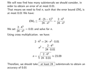
20. The error bound for Simpson’s rule with n points is
L · (5 − 1)5
ESn ≤
180 · n4
Here L = max|f (4) (x)|, where x ∈ [1, 5].
We compute the fourth derivative of f (x) = 1
x = x −1
f (x) = −x −2
f (x) = −(−2)x −3 = 2x −3
f (x) = 2(−3)x −4 = −6x −4
24
f (4) (x) = −6(−4)x −5 = 24x −5 =
x5
24
As x increases, x 5 decreases (the larger the denominator, the
smaller the fraction). Therefore, the largest value that 24 will take
x5
as x ranges from 1 to 5 is when x = 1, so L = 24 = 24. Then
13
24 · (5 − 1)5
ES4 ≤ ≈ 0.53
180 · 44
This shows that our estimate of 1.62 for the value of the integral
has an error of at most 0.53. This is not a very good estimate.

21. We will now find how many subintervals we should consider, in
order to obtain an error of at most 0.01.
That means we need to find n, such that the error bound ESn is at
most 0.01 L · (5 − 1)5 24 · 45
ESn ≤ =
180 · n4 180 · n4
24 · 45
We set = 0.01 and solve for n. Use cross-multiplication:
180 · n4
24 · 45 = 180 · n4 · 0.01
24 · 45
n4 =
180 · 0.01
4 24 · 45
n= ≈ 10.8
180 · 0.01
Therefore, we should take at least 12 subintervals (an even
number) to obtain an accuracy of 0.01
Note how much more efficient Simpson’s rule is, compared to the
other two methods (12 subintervals are needed to obtain the same
accuracy as the Midpoint rule would produce with 24 subintervals,
or as the Trapezoidal rule would produce with 33 subintervals).