Download as PDF, PPTX


![Probability Distribution (Population Based)
• Probability Density
Function (pdf) (p(x))
– Describes the probability
distribution of all possible
measures of x.
– Limiting case of the relative
frequency.
Probability Density Function
Probability per unit
change in x
0.3
• Probability Distribution
Function (P(x))
P x P[ X x]
X x
Probability that
– Probability Distribution
Function is the integral of
the pdf, i.e.
x
P x p x dx
0.25
Q: Plot the probability distribution function
vs x.
Q: What is the maximum value of P(x)?
0.2
0.15
0.1
0.05
0
30 35 40 45 50 55 60 65 70 75 80
x Value (Bin)
Slide 9](https://image.slidesharecdn.com/erroranalysis-statistics-140129181324-phpapp01/85/Error-analysis-statistics-9-320.jpg)
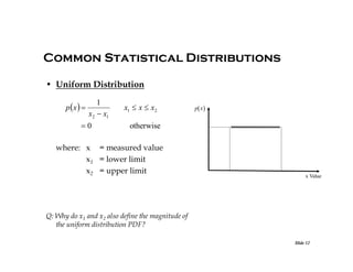
![Common Statistical Distributions
Ex: A voltage measurement has a Gaussian
distribution with mean 3.4 [V] and a
standard deviation of 0.4 [V]. Using
Chapter 4, Appendix A, calculate the
probability that a measurement is
between:
(a) [2.98, 3.82] [V]
Ex: The quantization error of an ADC has
a uniform distribution in the
quantization interval Q. What is the
probability that the actual input voltage
is within Q/8 of the estimated input
voltage?
(b) [2.4, 4.02] [V]
Slide 13](https://image.slidesharecdn.com/erroranalysis-statistics-140129181324-phpapp01/85/Error-analysis-statistics-13-320.jpg)
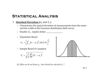
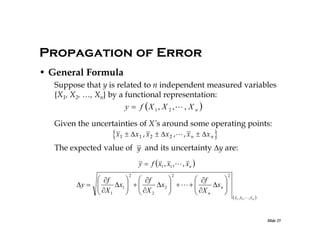
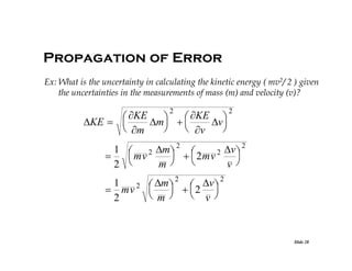
![Propagation of Error
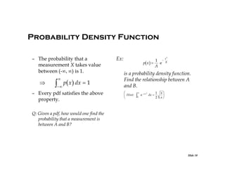
•Proof:
Assume that the variability in measurement y is caused
by k independent zero-mean error sources: e1, e2, . . . , ek.
Then, (y - ytrue)2 = (e1 + e2 + . . . + ek)2
= e12 + e22 + . . . + ek2 + 2e1e2 + 2e1e3 + . . .
E[(y - ytrue)2] = E[e12 + e22 + . . . + ek2 + 2e1e2 + 2e1e3 + . . .]
= E[e12 + e22 + . . . + ek2]
y
E e1 2 E e2 2 E e k 2 1 2 2 2 k 2
Slide 26](https://image.slidesharecdn.com/erroranalysis-statistics-140129181324-phpapp01/85/Error-analysis-statistics-26-320.jpg)
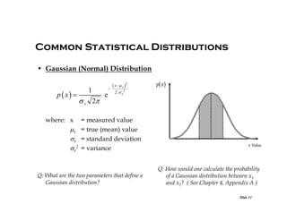
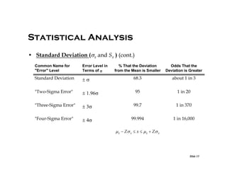
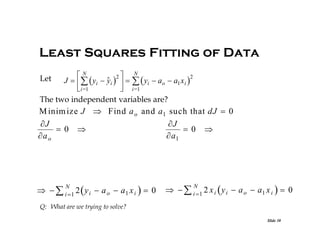
![• Best Linear Fit
–How do we characterize “BEST”?
Fit a linear model (relation)
Output Y
Least Squares Fitting of Data
best linear
fit yest
yi ao a1 xi
to N pairs of [xi, yi] measurements.
Given xi, the error between the
estimated output y i and the measured
output yi is:
ni yi yi
measured
output yi
Input X
The “BEST” fit is the model that
N 2
N
2
min ni min yi yi
minimizes the sum of the ___________
i=1
i=1
of the error
Least Square Error
Slide 29](https://image.slidesharecdn.com/erroranalysis-statistics-140129181324-phpapp01/85/Error-analysis-statistics-29-320.jpg)
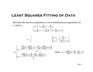
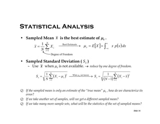
![Least Squares Fitting of Data
• Summary: Given N pairs of input/output measurements [xi, yi],
the best linear Least Squares model from input xi to output yi is:
yi ao a1 xi
x y x x y
2
where
ao
a1
i
i
i
i i
N x i yi x i yi
and N
x i 2 xi
• The process of minimizing squared error can be used for fitting
nonlinear models and many engineering applications.
• Same result can also be derived from a probability distribution
point of view (see Course Notes, Ch. 4 - Maximum Likelihood Estimation ).
Q: Given a theoretical model y = ao + a2 x2 , what are the Least Squares estimates for ao & a2?
Slide 32
2](https://image.slidesharecdn.com/erroranalysis-statistics-140129181324-phpapp01/85/Error-analysis-statistics-32-320.jpg)

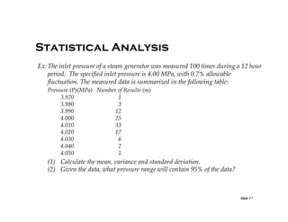
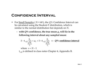
This document discusses concepts related to error analysis and statistics. It covers accuracy and precision, individual measurement uncertainty including means, variance, standard deviation and confidence intervals. It also discusses uncertainty when calculating quantities from multiple measurements using error propagation. Additionally, it discusses least squares fitting of data. Key points include how to quantify accuracy and precision, characterize the distribution of data, calculate uncertainty intervals, and propagate errors through calculations involving multiple measured variables.